Bellabeat Case Study
Updated: Mar 21, 2024
This case study is part of the Google Data Analytics Professional Certificate. It will focus on Bellabeat, a wellness brand for women, and provide analysis on smart device usage to inform and refine its marketing strategy. To achieve this the data analysis process will be followed: ask, prepare, process, analyse, share, and act. RStudio, a programming tool built for R, will be employed to clean, analyse and visualise the data.
Table of Contents
The Company: Bellabeat
Bellabeat is a wellness brand providing high-tech products and services designed to help women adopt healthier lifestyles.
Bellabeat was founded by Urška Sršen and Sando Mur in 2013 and has grown rapidly over the years. The company has extensively invested in both traditional and digital marketing, including Google search engines and maintaining an active social media presence. Despite its successes, Bellabeat recognizes the potential for further growth. Therefore, an in-depth analysis of consumer data from a different brand will be conducted to inform Bellabeat's marketing strategy and potentially enhance its existing products and features.
Products
Bellabeat App - Provides users with health data related to their activity, sleep, stress, menstrual cycle, and mindfulness habits, allowing users to understand their habits better and make healthier decisions.
Bellabeat Membership - Offers users 24/7 access to personalized guidance on nutrition, activity, sleep, health and beauty, and mindfulness tailored to their lifestyle and goals.
Leaf - A wearable wellness tracker available as a bracelet, necklace, or clip. It can track activity, sleep, and stress levels while also sending reminders to stay active.
Spring - A smart water bottle tracking daily water intake.
Time - A luxury wellness watch equipped with smart technology to monitor user’s activity, sleep, and stress levels, providing insight into users’ daily lifestyle and progress while sending reminders to stay active. Its elegant design makes the watch suitable for any occasion.
Ivy - A health tracker in the form of an elegant bracelet, monitoring not only activity, sleep, and stress but also heart rate, respiratory rate, cardiac coherence, and physical and mental activity.
Target Audience

Key Demographics
Age: 19 - 40; women in various life stages, from puberty to menopause
Gender: Female
Location: Primarily the USA, with additional markets in Europe, Asia, and the Middle East
Socio-economic Status: Middle and upper-class working professionals
Key Psychographics
They have a holistic view of health by caring for the whole person - the physical, mental, spiritual, and social well-being.
They are health-conscious, prioritising healthy dietary choices.
They tend to invest considerable money on health care and wellness.
Challenges and Needs
Limited time for daily workouts due to a typical 5-day workweek.
Desire for fitness trackers that are functional, sleek, and stylish, suitable for any occasion.
Section 1: Ask
In this section, the problem to be solved will be defined.
1.1 Business Task
Bellabeat aims to identify potential growth opportunities by analyzing smart device usage data to understand how consumers use non-Bellabeat smart devices. Insights gained will guide Bellabeat's marketing strategy and inspire new ideas for their existing products and services.
This case study will focus on improving one of Bellabeat's products - Ivy, the wellness and health tracker.
Questions to Consider
What are the current trends in smart device usage?
How do these trends relate to Bellabeat's target customers?
How can these trends influence Bellabeat's marketing strategy?
1.2 Key Stakeholders
Urška Sršen - Co-founder and Chief Creative Officer of Bellabeat
Sando Mur - Co-founder and member of Bellabeat's executive team
Bellabeat Marketing Analytics Team
Section 2: Prepare
In this section, useful and relevant data for solving the business task will be identified.
2.1 Data Source and Data Organisation
Fort this case study, the FitBit Fitness Tracker Data will be used. The dataset is publicly available on Kaggle. The dataset was collected through a survey via Amazon Mechanical Turk between March 12, 2016, and May 12, 2016. It contains personal tracker data from 30 Fitbit users, who consented to submit minute-level output for physical activity, heart rate, and sleep monitoring. This includes information on daily activity, steps, and heart rate, revealing patterns in users' habits. The dataset is organized into 18 CSV files in both long and wide formats.
2.2 Data Licensing and Privacy
The dataset is published by Möbius under the CC0: Public Domain Creative License, allowing free use without requiring permission from the copyright owner. Therefore, no licensing for the dataset is needed for this analysis.
Participants provided consent for the submission of personal tracker data, and their identities were anonymized using ID numbers instead of real names to ensure participant confidentiality.
2.3 ROCCC Analysis
To evaluate if the data source is credible and trustworthy, the ROCCC analysis will be employed.
Reliable: Low
The dataset includes only 30 participants, which may not adequately represent Fitbit's user base, which is more than 31 million in 2020. While the sample size is small, according to the Central Limit Theorem (CLT), the sample of 30 is the smallest size that is still considered valid. However, a larger sample size would still be recommended to increase the confidence level of the research.
The survey was conducted over two months, from 03/12/2016 to 05/12/2016, but the data only shows one month of activity from 04/12/2016 to 05/12/2016. While some people might have daily fitness routines, many people might adjust their fitness routine throughout the seasons. One month of data might not reflect that adjustment. A longer timeframe, spanning a full year, would offer more comprehensive insights.
Amazon Mechanical Turk is known to resemble the US population fairly well, relevant to this study as Bellabeat's customers are predominantly Americans.
Original: Low
Third-party data from Amazon Mechanical Turk was used. While this company is commonly used for behavioral research, direct data from Fitbit would bolster reliability.
Comprehensive: Medium
The dataset includes information about activity, sleep, steps, and heart rate, relevant to understanding smart device usage trends.
Bellabeat's target market is women. Therefore, data related specifically to women's health and activity would be beneficial to find trends that could be applied to Bellabeat's customers.
The dataset focuses solely on Fitbit data. However, there are many other fitness smart device companies with different functionalities and services, which could provide additional insights.
Current: Low
The study was conducted in 2016, which was 7 years ago. Since then, fitness trends have evolved significantly, especially after Covid-19. For instance, outdoor activities surged in popularity, and home exercise gyms became more prevalent, trends that were not prominent in 2016.
Wearable fitness technology was the no.1 trend in both 2016 and 2022. However, during that period, health and fitness technology have developed immensely, with many new services and functions being provided.
These changes may decrease the usefulness and relevance of the data, potentially rendering it insufficient for current analysis.
Cited: High
The data is cited with sources being documented.
Data was collected by a third-party company, Amazon Mechanical Turk, made available through Möbius.
The dataset was last updated 3 years ago.
2.4 Limitations
No demographic characteristics about the participants were collected, such as their gender, age, location, and lifestyle. Without this information, it's challenging to determine if the dataset accurately represents Bellabeat's target audience.
It is also unknown how the data was collected. Whether random sampling or purposive sampling was utilized.
Section 3: Process
In this section, the selected data will be cleaned to ensure it is complete and free of errors and outliers. RStudio will be used to explore, analyze, and visualize the data.
3.1 Installing and Loading Packages
First, key packages for the analysis will be installed and then loaded to use their functionalities.
# Installing packages
install.packages("tidyverse") #for transforming and presenting data
install.packages("dplyr") #for data manipulation
install.packages("readr") #to read rectangular data
install.packages("janitor") #for examining and cleaning data
install.packages("ggplot2") #to create plots
install.packages("lubridate") #to work with dates and times
install.packages("skimr") #to provide summary statistics
install.packages("gridExtra") #to arrange multiple plots on a page
install.packages("ggpubr") #to create and customise ggplot2-based graphs

# Loading libraries
library("tidyverse")
library("dplyr")
library("readr")
library("janitor")
library("ggplot2")
library("lubridate")
library("skimr")
library("gridExtra")
library("ggpubr")
3.2 Importing Datasets and Assigning New Names
Before importing the datasets, it is important to verify if they are in the current working directory. If not, the setwd() function will be utilised to change this. Following that, the datasets will be imported, and new names will be assigned to facilitate identification.
# Changing the working directory
setwd("/Users/thuhangtranova/Downloads/Fitabase Data 4.12.16-5.12.16")

# Importing datasets and assigning new names
daily_activity <- read_csv("dailyActivity_merged.csv")
daily_calories <- read_csv("dailyCalories_merged.csv")
daily_intensities <- read_csv("dailyIntensities_merged.csv")
daily_steps <- read_csv("dailySteps_merged.csv")
daily_sleep <- read_csv("sleepDay_merged.csv")
heartrate_seconds <- read_csv("heartrate_seconds_merged.csv")
hourly_calories <- read_csv("hourlyCalories_merged.csv")
hourly_intensities <- read_csv("hourlyIntensities_merged.csv")
hourly_steps <- read_csv("hourlySteps_merged.csv")
minute_calories_narrow <- read_csv("minuteCaloriesNarrow_merged.csv")
minute_calories_wide <- read_csv("minuteCaloriesWide_merged.csv")
minute_intensities_narrow <- read_csv("minuteIntensitiesNarrow_merged.csv")
minute_intensities_wide <- read_csv("minuteIntensitiesWide_merged.csv")
minute_METs_narrow <- read_csv("minuteMETsNarrow_merged.csv")
minute_sleep <- read_csv("minuteSleep_merged.csv")
minute_steps_narrow <- read_csv("minuteStepsNarrow_merged.csv")
minute_steps_wide <- read_csv("minuteStepsWide_merged.csv")
weight_log_info <- read_csv("weightLogInfo_merged.csv")
3.3 Exploring the Datasets
To get a quick idea of what is in the datasets, the glimpse() function will be used. The datasets will be divided into daily, hourly, minute, and second dataframes.
Daily DataFrames
# A quick preview of Daily Datasets
print("Daily Activity")
glimpse(daily_activity)

print("Daily Calories")
glimpse(daily_calories)

print("Daily Intensities")
glimpse(daily_intensities)

print("Daily Steps")
glimpse(daily_steps)

print("Daily Sleep")
glimpse(daily_sleep)

print("Weight Log Info")
glimpse(weight_log_info)
Output
[1] "Daily Activity"
Rows: 940
Columns: 15
$ Id                       <dbl> 1503960366, 1503960366, 1503960366, 1503960366, 1…
$ ActivityDate             <chr> "4/12/2016", "4/13/2016", "4/14/2016", "4/15/2016…
$ TotalSteps               <dbl> 13162, 10735, 10460, 9762, 12669, 9705, 13019, 15…
$ TotalDistance            <dbl> 8.50, 6.97, 6.74, 6.28, 8.16, 6.48, 8.59, 9.88, 6…
$ TrackerDistance          <dbl> 8.50, 6.97, 6.74, 6.28, 8.16, 6.48, 8.59, 9.88, 6…
$ LoggedActivitiesDistance <dbl> 0, 0, 0, 0, 0, 0, 0, 0, 0, 0, 0, 0, 0, 0, 0, 0, 0…
$ VeryActiveDistance       <dbl> 1.88, 1.57, 2.44, 2.14, 2.71, 3.19, 3.25, 3.53, 1…
$ ModeratelyActiveDistance <dbl> 0.55, 0.69, 0.40, 1.26, 0.41, 0.78, 0.64, 1.32, 0…
$ LightActiveDistance      <dbl> 6.06, 4.71, 3.91, 2.83, 5.04, 2.51, 4.71, 5.03, 4…
$ SedentaryActiveDistance  <dbl> 0, 0, 0, 0, 0, 0, 0, 0, 0, 0, 0, 0, 0, 0, 0, 0, 0…
$ VeryActiveMinutes        <dbl> 25, 21, 30, 29, 36, 38, 42, 50, 28, 19, 66, 41, 3…
$ FairlyActiveMinutes      <dbl> 13, 19, 11, 34, 10, 20, 16, 31, 12, 8, 27, 21, 5,…
$ LightlyActiveMinutes     <dbl> 328, 217, 181, 209, 221, 164, 233, 264, 205, 211,…
$ SedentaryMinutes         <dbl> 728, 776, 1218, 726, 773, 539, 1149, 775, 818, 83…
$ Calories                 <dbl> 1985, 1797, 1776, 1745, 1863, 1728, 1921, 2035, 1…

[1] "Daily Calories"
Rows: 940
Columns: 3
$ Id          <dbl> 1503960366, 1503960366, 1503960366, 1503960366, 1503960366, 15…
$ ActivityDay <chr> "4/12/2016", "4/13/2016", "4/14/2016", "4/15/2016", "4/16/2016…
$ Calories    <dbl> 1985, 1797, 1776, 1745, 1863, 1728, 1921, 2035, 1786, 1775, 18…

[1] "Daily Intensities"
Rows: 940
Columns: 10
$ Id                       <dbl> 1503960366, 1503960366, 1503960366, 1503960366, 1…
$ ActivityDay              <chr> "4/12/2016", "4/13/2016", "4/14/2016", "4/15/2016…
$ SedentaryMinutes         <dbl> 728, 776, 1218, 726, 773, 539, 1149, 775, 818, 83…
$ LightlyActiveMinutes     <dbl> 328, 217, 181, 209, 221, 164, 233, 264, 205, 211,…
$ FairlyActiveMinutes      <dbl> 13, 19, 11, 34, 10, 20, 16, 31, 12, 8, 27, 21, 5,…
$ VeryActiveMinutes        <dbl> 25, 21, 30, 29, 36, 38, 42, 50, 28, 19, 66, 41, 3…
$ SedentaryActiveDistance  <dbl> 0, 0, 0, 0, 0, 0, 0, 0, 0, 0, 0, 0, 0, 0, 0, 0, 0…
$ LightActiveDistance      <dbl> 6.06, 4.71, 3.91, 2.83, 5.04, 2.51, 4.71, 5.03, 4…
$ ModeratelyActiveDistance <dbl> 0.55, 0.69, 0.40, 1.26, 0.41, 0.78, 0.64, 1.32, 0…
$ VeryActiveDistance       <dbl> 1.88, 1.57, 2.44, 2.14, 2.71, 3.19, 3.25, 3.53, 1…

[1] "Daily Steps"
Rows: 940
Columns: 3
$ Id          <dbl> 1503960366, 1503960366, 1503960366, 1503960366, 1503960366, 15…
$ ActivityDay <chr> "4/12/2016", "4/13/2016", "4/14/2016", "4/15/2016", "4/16/2016…
$ StepTotal   <dbl> 13162, 10735, 10460, 9762, 12669, 9705, 13019, 15506, 10544, 9…

[1] "Daily Sleep"
Rows: 413
Columns: 5
$ Id                 <dbl> 1503960366, 1503960366, 1503960366, 1503960366, 1503960…
$ SleepDay           <chr> "4/12/2016 12:00:00 AM", "4/13/2016 12:00:00 AM", "4/15…
$ TotalSleepRecords  <dbl> 1, 2, 1, 2, 1, 1, 1, 1, 1, 1, 1, 1, 1, 1, 1, 1, 1, 1, 1…
$ TotalMinutesAsleep <dbl> 327, 384, 412, 340, 700, 304, 360, 325, 361, 430, 277, …
$ TotalTimeInBed     <dbl> 346, 407, 442, 367, 712, 320, 377, 364, 384, 449, 323, …

[1] "Weight Log Info"
Rows: 67
Columns: 8
$ Id             <dbl> 1503960366, 1503960366, 1927972279, 2873212765, 2873212765,…
$ Date           <chr> "5/2/2016 11:59:59 PM", "5/3/2016 11:59:59 PM", "4/13/2016 …
$ WeightKg       <dbl> 52.6, 52.6, 133.5, 56.7, 57.3, 72.4, 72.3, 69.7, 70.3, 69.9…
$ WeightPounds   <dbl> 115.9631, 115.9631, 294.3171, 125.0021, 126.3249, 159.6147,…
$ Fat            <dbl> 22, NA, NA, NA, NA, 25, NA, NA, NA, NA, NA, NA, NA, NA, NA,…
$ BMI            <dbl> 22.65, 22.65, 47.54, 21.45, 21.69, 27.45, 27.38, 27.25, 27.…
$ IsManualReport <lgl> TRUE, TRUE, FALSE, TRUE, TRUE, TRUE, TRUE, TRUE, TRUE, TRUE…
$ LogId          <dbl> 1.462234e+12, 1.462320e+12, 1.460510e+12, 1.461283e+12, 1.4…
Hourly DataFrames
# A quick preview of Hourly Datasets
print("Hourly Calories")
glimpse(hourly_calories)

print("Hourly Intensities")
glimpse(hourly_intensities)

print("Hourly Steps")
glimpse(hourly_steps)
Output
[1] "Hourly Calories"
Rows: 22,099
Columns: 3
$ Id           <dbl> 1503960366, 1503960366, 1503960366, 1503960366, 1503960366, 1…
$ ActivityHour <chr> "4/12/2016 12:00:00 AM", "4/12/2016 1:00:00 AM", "4/12/2016 2…
$ Calories     <dbl> 81, 61, 59, 47, 48, 48, 48, 47, 68, 141, 99, 76, 73, 66, 110,…

[1] "Hourly Intensities"
Rows: 22,099
Columns: 4
$ Id               <dbl> 1503960366, 1503960366, 1503960366, 1503960366, 150396036…
$ ActivityHour     <chr> "4/12/2016 12:00:00 AM", "4/12/2016 1:00:00 AM", "4/12/20…
$ TotalIntensity   <dbl> 20, 8, 7, 0, 0, 0, 0, 0, 13, 30, 29, 12, 11, 6, 36, 58, 1…
$ AverageIntensity <dbl> 0.333333, 0.133333, 0.116667, 0.000000, 0.000000, 0.00000…

[1] "Hourly Steps"
Rows: 22,099
Columns: 3
$ Id           <dbl> 1503960366, 1503960366, 1503960366, 1503960366, 1503960366, 1…
$ ActivityHour <chr> "4/12/2016 12:00:00 AM", "4/12/2016 1:00:00 AM", "4/12/2016 2…
$ StepTotal    <dbl> 373, 160, 151, 0, 0, 0, 0, 0, 250, 1864, 676, 360, 253, 221, …
Minute DataFrames
# A quick preview of Minute Datasets
print("Minute Calories")
glimpse(minute_calories_narrow)

print("Minute Intensities")
glimpse(minute_intensities_narrow)

print("Minute METs")
glimpse(minute_METs_narrow)

print("Minute Sleep")
glimpse(minute_sleep)

print("Minute Steps")
glimpse(minute_steps_narrow)
Output
[1] "Minute Calories"
Rows: 1,325,580
Columns: 3
$ Id             <dbl> 1503960366, 1503960366, 1503960366, 1503960366, 1503960366,…
$ ActivityMinute <chr> "4/12/2016 12:00:00 AM", "4/12/2016 12:01:00 AM", "4/12/201…
$ Calories       <dbl> 0.7865, 0.7865, 0.7865, 0.7865, 0.7865, 0.9438, 0.9438, 0.9…

[1] "Minute Intensities"
Rows: 1,325,580
Columns: 3
$ Id             <dbl> 1503960366, 1503960366, 1503960366, 1503960366, 1503960366,…
$ ActivityMinute <chr> "4/12/2016 12:00:00 AM", "4/12/2016 12:01:00 AM", "4/12/201…
$ Intensity      <dbl> 0, 0, 0, 0, 0, 0, 0, 0, 0, 0, 0, 0, 0, 0, 0, 0, 0, 0, 0, 0,…

[1] "Minute METs"
Rows: 1,325,580
Columns: 3
$ Id             <dbl> 1503960366, 1503960366, 1503960366, 1503960366, 1503960366,…
$ ActivityMinute <chr> "4/12/2016 12:00:00 AM", "4/12/2016 12:01:00 AM", "4/12/201…
$ METs           <dbl> 10, 10, 10, 10, 10, 12, 12, 12, 12, 12, 12, 12, 10, 10, 12,…

[1] "Minute Sleep"
Rows: 188,521
Columns: 4
$ Id    <dbl> 1503960366, 1503960366, 1503960366, 1503960366, 1503960366, 15039603…
$ date  <chr> "4/12/2016 2:47:30 AM", "4/12/2016 2:48:30 AM", "4/12/2016 2:49:30 A…
$ value <dbl> 3, 2, 1, 1, 1, 1, 1, 2, 2, 2, 3, 3, 3, 3, 3, 2, 1, 1, 1, 1, 1, 1, 1,…
$ logId <dbl> 11380564589, 11380564589, 11380564589, 11380564589, 11380564589, 113…

[1] "Minute Steps"
Rows: 1,325,580
Columns: 3
$ Id             <dbl> 1503960366, 1503960366, 1503960366, 1503960366, 1503960366,…
$ ActivityMinute <chr> "4/12/2016 12:00:00 AM", "4/12/2016 12:01:00 AM", "4/12/201…
$ Steps          <dbl> 0, 0, 0, 0, 0, 0, 0, 0, 0, 0, 0, 0, 0, 0, 0, 0, 0, 0, 0, 0,…
Second DataFrames
# A quick preview of Second Datasets
print("Heartrate Seconds")
glimpse(heartrate_seconds)
Output
[1] "Heartrate Seconds"
Rows: 2,483,658
Columns: 3
$ Id    <dbl> 2022484408, 2022484408, 2022484408, 2022484408, 2022484408, 20224844…
$ Time  <chr> "4/12/2016 7:21:00 AM", "4/12/2016 7:21:05 AM", "4/12/2016 7:21:10 A…
$ Value <dbl> 97, 102, 105, 103, 101, 95, 91, 93, 94, 93, 92, 89, 83, 61, 60, 61, …
3.4 Data Cleaning
Following the exploration of the datasets, several issues have been identified necessitating data cleaning actions to ensure data integrity and prepare the data for analysis.
3.4.1 Naming Conventions and Date Variable Formatting
Inconsistent naming conventions: With the exception of "minute_sleep", all dataframes adhere to the UpperCamelCase format. However, "minute_sleep" uses both UpperCamelCase and lowercase formats. → All variable names will be standardised to follow the snake_case naming convention using the clean_names() function. This will make all the variable names consistent and easier to read.
Different names for variables with the same meaning: Although most columns with variables of the same meaning share consistent titles across all dataframes (e.g., "Id"), the date columns exhibit variations such as "ActivityDate," "ActivityDay," and "Time." → These variables will be renamed to follow the same title "activity_date." This will be helpful later during merging.
Date Column's Data Type: Currently, the date column is stored as a character type, which poses challenges for analysis. To address this, new columns will be created where the date will be converted into either date or date-time format using the mdy() and mdy_hms() functions. This standardized date-time formatting will ensure consistency across all datasets.
Daily DataFrames
# Naming conventions and date variable formatting of Daily DataFrames
clean_daily_activity <- daily_activity %>%
  clean_names()
clean_daily_activity$activity_date_ymd <- mdy(clean_daily_activity$activity_date)
print("Clean Daily Activity")
glimpse(clean_daily_activity)

clean_daily_calories <- daily_calories %>%
  rename(activity_date = ActivityDay) %>%
  clean_names()
clean_daily_calories$activity_date_ymd <- mdy(clean_daily_calories$activity_date)
print("Clean Daily Calories")
glimpse(clean_daily_calories)

clean_daily_intensities <- daily_intensities %>%
  rename(activity_date = ActivityDay) %>%
  clean_names()
clean_daily_intensities$activity_date_ymd <- mdy(clean_daily_intensities$activity_date)
print("Clean Daily Intensities")
glimpse(clean_daily_intensities)

clean_daily_steps <- daily_steps %>%
  rename(activity_date = ActivityDay,
         total_steps = StepTotal) %>%
  clean_names()
clean_daily_steps$activity_date_ymd <- mdy(clean_daily_steps$activity_date)
print("Clean Daily Steps")
glimpse(clean_daily_steps)

clean_daily_sleep <- daily_sleep %>%
  rename(activity_date = SleepDay) %>%
  clean_names()
clean_daily_sleep$activity_date_ymd <- mdy_hms(clean_daily_sleep$activity_date, tz=Sys.timezone())
print("Clean Daily Sleep")
glimpse(clean_daily_sleep)

clean_weight_log_info <- weight_log_info %>%
  rename(activity_date = Date,
         weight_kg = WeightKg,
         weight_lb = WeightPounds,
         manual_report = IsManualReport) %>%
  clean_names()
clean_weight_log_info$activity_date_ymdhms <- mdy_hms(clean_weight_log_info$activity_date, tz=Sys.timezone())
print("Clean Weight Log Info")
glimpse(clean_weight_log_info)
Output
[1] "Clean Daily Calories"
Rows: 940
Columns: 4
$ id                <dbl> 1503960366, 1503960366, 1503960366, 1503960366, 15039…
$ activity_date     <chr> "4/12/2016", "4/13/2016", "4/14/2016", "4/15/2016", "…
$ calories          <dbl> 1985, 1797, 1776, 1745, 1863, 1728, 1921, 2035, 1786,…
$ activity_date_ymd <date> 2016-04-12, 2016-04-13, 2016-04-14, 2016-04-15, 2016…

[1] "Clean Daily Intensities"
Rows: 940
Columns: 11
$ id                         <dbl> 1503960366, 1503960366, 1503960366, 15039603…
$ activity_date              <chr> "4/12/2016", "4/13/2016", "4/14/2016", "4/15…
$ sedentary_minutes          <dbl> 728, 776, 1218, 726, 773, 539, 1149, 775, 81…
$ lightly_active_minutes     <dbl> 328, 217, 181, 209, 221, 164, 233, 264, 205,…
$ fairly_active_minutes      <dbl> 13, 19, 11, 34, 10, 20, 16, 31, 12, 8, 27, 2…
$ very_active_minutes        <dbl> 25, 21, 30, 29, 36, 38, 42, 50, 28, 19, 66, …
$ sedentary_active_distance  <dbl> 0, 0, 0, 0, 0, 0, 0, 0, 0, 0, 0, 0, 0, 0, 0,…
$ light_active_distance      <dbl> 6.06, 4.71, 3.91, 2.83, 5.04, 2.51, 4.71, 5.…
$ moderately_active_distance <dbl> 0.55, 0.69, 0.40, 1.26, 0.41, 0.78, 0.64, 1.…
$ very_active_distance       <dbl> 1.88, 1.57, 2.44, 2.14, 2.71, 3.19, 3.25, 3.…
$ activity_date_ymd          <date> 2016-04-12, 2016-04-13, 2016-04-14, 2016-04…

[1] "Clean Daily Steps"
Rows: 940
Columns: 4
$ id                <dbl> 1503960366, 1503960366, 1503960366, 1503960366, 15039…
$ activity_date     <chr> "4/12/2016", "4/13/2016", "4/14/2016", "4/15/2016", "…
$ total_steps       <dbl> 13162, 10735, 10460, 9762, 12669, 9705, 13019, 15506,…
$ activity_date_ymd <date> 2016-04-12, 2016-04-13, 2016-04-14, 2016-04-15, 2016…

[1] "Clean Daily Sleep"
Rows: 413
Columns: 6
$ id                   <dbl> 1503960366, 1503960366, 1503960366, 1503960366, 15…
$ activity_date        <chr> "4/12/2016 12:00:00 AM", "4/13/2016 12:00:00 AM", …
$ total_sleep_records  <dbl> 1, 2, 1, 2, 1, 1, 1, 1, 1, 1, 1, 1, 1, 1, 1, 1, 1,…
$ total_minutes_asleep <dbl> 327, 384, 412, 340, 700, 304, 360, 325, 361, 430, …
$ total_time_in_bed    <dbl> 346, 407, 442, 367, 712, 320, 377, 364, 384, 449, …
$ activity_date_ymd    <dttm> 2016-04-12, 2016-04-13, 2016-04-15, 2016-04-16, 2…

[1] "Clean Weight Log Info"
Rows: 67
Columns: 9
$ id                   <dbl> 1503960366, 1503960366, 1927972279, 2873212765, 28…
$ activity_date        <chr> "5/2/2016 11:59:59 PM", "5/3/2016 11:59:59 PM", "4…
$ weight_kg            <dbl> 52.6, 52.6, 133.5, 56.7, 57.3, 72.4, 72.3, 69.7, 7…
$ weight_lb            <dbl> 115.9631, 115.9631, 294.3171, 125.0021, 126.3249, …
$ fat                  <dbl> 22, NA, NA, NA, NA, 25, NA, NA, NA, NA, NA, NA, NA…
$ bmi                  <dbl> 22.65, 22.65, 47.54, 21.45, 21.69, 27.45, 27.38, 2…
$ manual_report        <lgl> TRUE, TRUE, FALSE, TRUE, TRUE, TRUE, TRUE, TRUE, T…
$ log_id               <dbl> 1.462234e+12, 1.462320e+12, 1.460510e+12, 1.461283…
$ activity_date_ymdhms <dttm> 2016-05-02 23:59:59, 2016-05-03 23:59:59, 2016-04…
Hourly DataFrames
# Naming conventions and date variable formatting of Hourly DataFrames
clean_hourly_calories <- hourly_calories %>%
  clean_names()
clean_hourly_calories$activity_hour_ymdhms <- mdy_hms(clean_hourly_calories$activity_hour, tz=Sys.timezone())
print("Clean Hourly Calories")
glimpse(clean_hourly_calories)

clean_hourly_intensities <- hourly_intensities %>%
  clean_names()
clean_hourly_intensities$activity_hour_ymdhms <- mdy_hms(clean_hourly_intensities$activity_hour, tz=Sys.timezone())
print("Clean Hourly Intensities")
glimpse(clean_hourly_intensities)

clean_hourly_steps <- hourly_steps %>%
  rename(total_steps = StepTotal) %>%
  clean_names()
clean_hourly_steps$activity_hour_ymdhms <- mdy_hms(clean_hourly_steps$activity_hour, tz=Sys.timezone())
print("Clean Hourly Steps")
glimpse(clean_hourly_steps)
Output
[1] "Clean Hourly Calories"
Rows: 22,099
Columns: 4
$ id                   <dbl> 1503960366, 1503960366, 1503960366, 1503960366, 15…
$ activity_hour        <chr> "4/12/2016 12:00:00 AM", "4/12/2016 1:00:00 AM", "…
$ calories             <dbl> 81, 61, 59, 47, 48, 48, 48, 47, 68, 141, 99, 76, 7…
$ activity_hour_ymdhms <dttm> 2016-04-12 00:00:00, 2016-04-12 01:00:00, 2016-04…

[1] "Clean Hourly Intensities"
Rows: 22,099
Columns: 5
$ id                   <dbl> 1503960366, 1503960366, 1503960366, 1503960366, 15…
$ activity_hour        <chr> "4/12/2016 12:00:00 AM", "4/12/2016 1:00:00 AM", "…
$ total_intensity      <dbl> 20, 8, 7, 0, 0, 0, 0, 0, 13, 30, 29, 12, 11, 6, 36…
$ average_intensity    <dbl> 0.333333, 0.133333, 0.116667, 0.000000, 0.000000, …
$ activity_hour_ymdhms <dttm> 2016-04-12 00:00:00, 2016-04-12 01:00:00, 2016-04…

[1] "Clean Hourly Steps"
Rows: 22,099
Columns: 4
$ id                   <dbl> 1503960366, 1503960366, 1503960366, 1503960366, 15…
$ activity_hour        <chr> "4/12/2016 12:00:00 AM", "4/12/2016 1:00:00 AM", "…
$ total_steps          <dbl> 373, 160, 151, 0, 0, 0, 0, 0, 250, 1864, 676, 360,…
$ activity_hour_ymdhms <dttm> 2016-04-12 00:00:00, 2016-04-12 01:00:00, 2016-04…
Minute DataFrames
# Naming conventions and date variabe formatting of Minute DataFrames
clean_minute_calories <- minute_calories_narrow %>%
  clean_names()
clean_minute_calories$activity_minute_ymdhms <- mdy_hms(clean_minute_calories$activity_minute, tz=Sys.timezone())
print("Clean Minute Calories")
glimpse(clean_minute_calories)

clean_minute_intensities <- minute_intensities_narrow %>%
  clean_names()
clean_minute_intensities$activity_minute_ymdhms <- mdy_hms(clean_minute_intensities$activity_minute, tz=Sys.timezone())
print("Clean Minute Intensities")
glimpse(clean_minute_intensities)

clean_minute_METs <- minute_METs_narrow %>%
  rename(mets = METs) %>%
  clean_names()
clean_minute_METs$activity_minute_ymdhms <- mdy_hms(clean_minute_METs$activity_minute, tz=Sys.timezone())
print("Clean Minute METs")
glimpse(clean_minute_METs)

clean_minute_sleep <- minute_sleep %>%
  rename(activity_minute = date,
         sleep_state = value) %>%
  clean_names()
clean_minute_sleep$activity_minute_ymdhms <- mdy_hms(clean_minute_sleep$activity_minute, tz=Sys.timezone())
print("Clean Minute Sleep")
glimpse(clean_minute_sleep)

clean_minute_steps <- minute_steps_narrow %>%
  rename(total_steps = Steps) %>%
  clean_names()
clean_minute_steps$activity_minute_ymdhms <- mdy_hms(clean_minute_steps$activity_minute, tz=Sys.timezone())
print("Clean Minute Steps")
glimpse(clean_minute_steps)
Output
[1] "Clean Minute Calories"
Rows: 1,325,580
Columns: 4
$ id                     <dbl> 1503960366, 1503960366, 1503960366, 1503960366, …
$ activity_minute        <chr> "4/12/2016 12:00:00 AM", "4/12/2016 12:01:00 AM"…
$ calories               <dbl> 0.7865, 0.7865, 0.7865, 0.7865, 0.7865, 0.9438, …
$ activity_minute_ymdhms <dttm> 2016-04-12 00:00:00, 2016-04-12 00:01:00, 2016-…

[1] "Clean Minute Intensities"
Rows: 1,325,580
Columns: 4
$ id                     <dbl> 1503960366, 1503960366, 1503960366, 1503960366, …
$ activity_minute        <chr> "4/12/2016 12:00:00 AM", "4/12/2016 12:01:00 AM"…
$ intensity              <dbl> 0, 0, 0, 0, 0, 0, 0, 0, 0, 0, 0, 0, 0, 0, 0, 0, …
$ activity_minute_ymdhms <dttm> 2016-04-12 00:00:00, 2016-04-12 00:01:00, 2016-…

[1] "Clean Minute METs"
Rows: 1,325,580
Columns: 4
$ id                     <dbl> 1503960366, 1503960366, 1503960366, 1503960366, …
$ activity_minute        <chr> "4/12/2016 12:00:00 AM", "4/12/2016 12:01:00 AM"…
$ mets                  <dbl> 10, 10, 10, 10, 10, 12, 12, 12, 12, 12, 12, 12, …
$ activity_minute_ymdhms <dttm> 2016-04-12 00:00:00, 2016-04-12 00:01:00, 2016-…

[1] "Clean Minute Sleep"
Rows: 188,521
Columns: 5
$ id                     <dbl> 1503960366, 1503960366, 1503960366, 1503960366, …
$ activity_minute        <chr> "4/12/2016 2:47:30 AM", "4/12/2016 2:48:30 AM", …
$ sleep_state            <dbl> 3, 2, 1, 1, 1, 1, 1, 2, 2, 2, 3, 3, 3, 3, 3, 2, …
$ log_id                 <dbl> 11380564589, 11380564589, 11380564589, 113805645…
$ activity_minute_ymdhms <dttm> 2016-04-12 02:47:30, 2016-04-12 02:48:30, 2016-…

[1] "Clean Minute Steps"
Rows: 1,325,580
Columns: 5
$ id                      <dbl> 1503960366, 1503960366, 1503960366, 1503960366,…
$ activity_minute         <chr> "4/12/2016 12:00:00 AM", "4/12/2016 12:01:00 AM…
$ total_steps             <dbl> 0, 0, 0, 0, 0, 0, 0, 0, 0, 0, 0, 0, 0, 0, 0, 0,…
$ activity_minute_ymdhms  <dttm> 2016-04-12 00:00:00, 2016-04-12 00:01:00, 2016…
Second DataFrame
# Naming conventions and date variable formatting of Second DataFrame
clean_heartrate_seconds <- heartrate_seconds %>%
  rename(activity_second = Time,
         heartrate = Value) %>%
  clean_names()
clean_heartrate_seconds$activity_second_ymdhms <- mdy_hms(clean_heartrate_seconds$activity_second, tz=Sys.timezone())
print("Clean Heartrate Seconds")
glimpse(clean_heartrate_seconds)
Output
[1] "Clean Heartrate Seconds"
Rows: 2,483,658
Columns: 5
$ id                      <dbl> 2022484408, 2022484408, 2022484408, 2022484408,…
$ activity_second         <chr> "4/12/2016 7:21:00 AM", "4/12/2016 7:21:05 AM",…
$ heartrate               <dbl> 97, 102, 105, 103, 101, 95, 91, 93, 94, 93, 92,…
$ activity_second_ymdhms  <dttm> 2016-04-12 07:21:00, 2016-04-12 07:21:05, 2016…
3.4.2. Unique Participant IDs
According to the data description, each dataset should contain 30 unique participant IDs. To verify this, the number of unique participants will be assessed using the n_unique() function.
Daily DataFrames
# Unique participant IDs: Daily DataFrames
print("Daily Activity")
n_unique(clean_daily_activity$id)

print("Daily Calories")
n_unique(clean_daily_calories$id)

print("Daily Intensities")
n_unique(clean_daily_intensities$id)

print("Daily Steps")
n_unique(clean_daily_steps$id)

print("Daily Sleep")
n_unique(clean_daily_sleep$id)

print("Daily Weight Log Info")
n_unique(clean_weight_log_info$id)
Output
[1] "Daily Calories"
[1] 33

[1] "Daily Intensities"
[1] 33

[1] "Daily Steps"
[1] 33

[1] "Daily Sleep"
[1] 24

[1] "Daily Weight Log Info"
[1] 8
Hourly DataFrames
# Unique participant IDs: Hourly DataFrames
print("Hourly Calories")
n_unique(clean_hourly_calories$id)

print("Hourly Intensities")
n_unique(clean_hourly_intensities$id)

print("Hourly Steps")
n_unique(clean_hourly_steps$id)
Output
[1] "Hourly Calories"
[1] 33

[1] "Hourly Intensities"
[1] 33

[1] "Hourly Steps"
[1] 33
Minute DataFrames
# Unique participant IDs: Minute DataFrames
print("Minute Calories")
n_unique(clean_minute_calories$id)

print("Minute Intensities")
n_unique(clean_minute_intensities$id)

print("Minute METs")
n_unique(clean_minute_METs$id)

print("Minute Sleep")
n_unique(clean_minute_sleep$id)

print("Minute Steps")
n_unique(clean_minute_steps$id)
Output
[1] "Minute Calories"
[1] 33

[1] "Minute Intensities"
[1] 33

[1] "Minute METs"
[1] 33

[1] "Minute Sleep"
[1] 24

[1] "Minute Steps"
[1] 33
Second DataFrame
# Unique participant IDs: Second DataFrame
print("Second Heartrate")
n_unique(clean_heartrate_seconds$id)
Output
[1] "Second Heartrate"
[1] 14
Observation
Based on the results, the datasets appear to be inconsistent with the author's description, showing predominantly 33 distinct IDs, three more than expected.
Most datasets have 33 participants, except for sleep (24), weight (8), and heart rate (14). This discrepancy implies that sleep, weight, and heart rate datasets are incomplete. This inconsistency might be because tracked activities are being automatically recognised and recorded by the device through movement. Unlike activities, weight measurements require manual entry into Fitbit, while heart rate tracking may necessitate user activation. Consequently, participants may not have consistently recorded their weight or activated heart rate tracking, leading to incomplete datasets.
Actions Taken
Given the limited participant counts in the weight (8) and heart datasets (14), these datasets will be excluded from further analysis as the sample size is not significant enough to make any conclusions.
3.4.3. Number of Active Days
Each dataset is expected to span 31 days. To confirm this, the number of active days in each dataset will be assessed using the n_unique() function.
Daily DataFrames
# Unique number of active days: Daily DataFrames
print("Daily Activity")
n_unique(clean_daily_activity$activity_date_ymd)

print("Daily Calories")
n_unique(clean_daily_calories$activity_date_ymd)

print("Daily Intensities")
n_unique(clean_daily_intensities$activity_date_ymd)

print("Daily Steps")
n_unique(clean_daily_steps$activity_date_ymd)

print("Daily Sleep")
n_unique(clean_daily_sleep$activity_date_ymd)
Output
[1] "Daily Activity"
[1] 31

[1] "Daily Calories"
[1] 31

[1] "Daily Intensities"
[1] 31

[1] "Daily Steps"
[1] 31

[1] "Daily Sleep"
[1] 31
Hourly DataFrames
# Unique number of active days: Hourly DataFrames
print("Hourly Calories")
n_unique(date(clean_hourly_calories$activity_hour_ymdhms))

print("Hourly Intensities")
n_unique(date(clean_hourly_intensities$activity_hour_ymdhms))

print("Hourly Steps")
n_unique(date(clean_hourly_steps$activity_hour_ymdhms))
Output
[1] "Hourly Calories"
[1] 31

[1] "Hourly Intensities"
[1] 31

[1] "Hourly Steps"
[1] 31
Minute DataFrames
# Unique number of active days: Minute DataFrames
print("Minute Calories")
n_unique(date(clean_minute_calories$activity_minute_ymdhms))

print("Minute Intensities")
n_unique(date(clean_minute_intensities$activity_minute_ymdhms))

print("Minute METs")
n_unique(date(clean_minute_METs$activity_minute_ymdhms))

print("Minute Sleep")
n_unique(date(clean_minute_sleep$activity_minute_ymdhms))

print("Minute Steps")
n_unique(date(clean_minute_steps$activity_minute_ymdhms))
Output
[1] "Minute Calories"
[1] 31

[1] "Minute Intensities"
[1] 31

[1] "Minute METs"
[1] 31

[1] "Minute Sleep"
[1] 32

[1] "Minute Steps"
[1] 31
Observation
Most datasets exhibit 31 active days, aligning with the expected duration of the research period. However, the "minute_sleep" dataset displays 32 active days. The research was supposed to start on 04/12/2016 and end 05/12/2016 (= 31 days). However, some participants went to bed before 12am on 04/11/2016; therefore, that date was also included in the data, amounting to 32 days.
3.4.4 Participants' Logged Activity
To ensure participant engagement throughout the entire 31-day research period, the number of logged activities will be examined.
clean_daily_activity %>%
  group_by(id) %>%
  count() %>%
  arrange(n) %>%
  tibble() %>%
  print(n=33)
Output
# A tibble: 33 × 2
           id     n
        <dbl> <int>
 1 4057192912     4
 2 2347167796    18
 3 8253242879    19
 4 3372868164    20
 5 6775888955    26
 6 7007744171    26
 7 6117666160    28
 8 6290855005    29
 9 8792009665    29
10 1644430081    30
11 3977333714    30
12 5577150313    30
13 1503960366    31
14 1624580081    31
15 1844505072    31
16 1927972279    31
17 2022484408    31
18 2026352035    31
19 2320127002    31
20 2873212765    31
21 4020332650    31
22 4319703577    31
23 4388161847    31
24 4445114986    31
25 4558609924    31
26 4702921684    31
27 5553957443    31
28 6962181067    31
29 7086361926    31
30 8053475328    31
31 8378563200    31
32 8583815059    31
33 8877689391    31
Observation
Participant with ID# 4057192912 has only 4 logged activities, which is significantly low. Although considering removal, given the already limited participant pool, the participant's data will be kept.
3.4.5 Missing Values
The number of missing values in each dataset will be examined using the sum(is.na(x)) and which(is.na(x)) functions.
Daily DataFrames
# Checking for missing values: Daily DataFrames
print ("Daily Activity")
if (sum(is.na(clean_daily_activity)) !=0) {
  print("Position of missing values - ")
  which(is.na(clean_daily_activity))
} else {
  print("No missing values")
}

print("Daily Calories")
if (sum(is.na(clean_daily_calories)) !=0) {
  print("Position of missing values - ")
  which(is.na(clean_daily_calories))
} else {
  print("No missing values")
}

print("Daily Intensities")
if (sum(is.na(clean_daily_intensities)) !=0) {
  print("Position of missing values - ")
  which(is.na(clean_daily_intensities))
} else {
  print("No missing values")
}

print("Daily Steps")
if (sum(is.na(clean_daily_steps)) !=0) {
  print("Position of missing values - ")
  which(is.na(clean_daily_steps))
} else {
  print("No missing values")
}

print("Daily Sleep")
if (sum(is.na(clean_daily_sleep)) !=0) {
  print("Position of missing values - ")
  which(is.na(clean_daily_sleep))
} else {
  print("No missing values")
}
Output
[1] "Daily Activity"
[1] "No missing values"

[1] "Daily Calories"
[1] "No missing values"

[1] "Daily Intensities"
[1] "No missing values"

[1] "Daily Steps"
[1] "No missing values"

[1] "Daily Sleep"
[1] "No missing values"
Hourly DataFrames
# Checking for missing values: Hourly DataFrames
print("Hourly Calories")
if (sum(is.na(clean_hourly_calories)) !=0) {
  print("Position of missing values - ")
  which(is.na(clean_hourly_calories))
} else {
  print("No missing values")
}

print("Hourly Intensities")
if (sum(is.na(clean_hourly_intensities)) !=0) {
  print("Position of missing values - ")
  which(is.na(clean_hourly_intensities))
} else {
  print("No missing values")
}

print("Hourly Steps")
if (sum(is.na(clean_hourly_steps)) !=0) {
  print("Position of missing values - ")
  which(is.na(clean_hourly_steps))
} else {
  print("No missing values")
}
Output
[1] "Hourly Calories"
[1] "No missing values"

[1] "Hourly Intensities"
[1] "No missing values"

[1] "Hourly Steps"
[1] "No missing values"
Minute DataFrames
# Checking for missing values: Minute DataFrames
print("Minute Calories")
if (sum(is.na(clean_minute_calories)) !=0) {
  print("Position of missing values - ")
  which(is.na(clean_minute_calories))
} else {
  print("No missing values")
}

print("Minute Intensities")
if (sum(is.na(clean_minute_intensities)) !=0) {
  print("Position of missing values - ")
  which(is.na(clean_minute_intensities))
} else {
  print("No missing values")
}

print("Minute METs")
if (sum(is.na(clean_minute_METs)) !=0) {
  print("Position of missing values - ")
  which(is.na(clean_minute_METs))
} else {
  print("No missing values")
}

print("Minute Sleep")
if (sum(is.na(clean_minute_sleep)) !=0) {
  print("Position of missing values - ")
  which(is.na(clean_minute_sleep))
} else {
  print("No missing values")
}

print("Minute Steps")
if (sum(is.na(clean_minute_steps)) !=0) {
  print("Position of missing values - ")
  which(is.na(clean_minute_steps))
} else {
  print("No missing values")
}
Output
[1] "Minute Calories"
[1] "No missing values"

[1] "Minute Intensities"
[1] "No missing values"

[1] "Minute METs"
[1] "No missing values"

[1] "Minute Sleep"
[1] "No missing values"

[1] "Minute Steps"
[1] "No missing values"
Observation
There are no missing values.
3.4.6 Removing duplicates
Duplicate data can cause inaccurate reporting. To find out if there are any duplicates, the sum(duplicated()) function will be used.
Daily DataFrames
# Checking for duplicates: Daily DataFrames
print("Daily Activity")
sum(duplicated(clean_daily_activity))

print("Daily Calories")
sum(duplicated(clean_daily_calories))

print("Daily Intensities")
sum(duplicated(clean_daily_intensities))

print("Daily Steps")
sum(duplicated(clean_daily_steps))

print("Daily Sleep")
sum(duplicated(clean_daily_sleep))
Output
[1] "Daily Activity"
[1] 0

[1] "Daily Calories"
[1] 0

[1] "Daily Intensities"
[1] 0

[1] "Daily Steps"
[1] 0

[1] "Daily Sleep"
[1] 3
Hourly DataFrames
# Checking for duplicates: Hourly DataFrames
print("Hourly Calories")
sum(duplicated(clean_hourly_calories))

print("Hourly Intensities")
sum(duplicated(clean_hourly_intensities))

print("Hourly Steps")
sum(duplicated(clean_hourly_steps))
Output
[1] "Hourly Calories"
[1] 0

[1] "Hourly Intensities"
[1] 0

[1] "Hourly Steps"
[1] 0
Minute DataFrames
# Checking for duplicates: Minute DataFrames
print("Minute Calories")
sum(duplicated(clean_minute_calories))

print("Minute Intensities")
sum(duplicated(clean_minute_intensities))

print("Minute METs")
sum(duplicated(clean_minute_METs))

print("Minute Sleep")
sum(duplicated(clean_minute_sleep))

print("Minute Steps")
sum(duplicated(clean_minute_steps))
Output
[1] "Minute Calories"
[1] 0

[1] "Minute Intensities"
[1] 0

[1] "Minute METs"
[1] 0

[1] "Minute Sleep"
[1] 543

[1] "Minute Steps"
[1] 0
Observation
Duplicates have been identified in the "daily_sleep" and "minute_sleep" dataframes.
Actions Taken
To remove these duplicates, the !duplicated() function will be used.
# Removing duplicates from the "Daily Sleep" DataFrame
clean_daily_sleep <- clean_daily_sleep[!duplicated(clean_daily_sleep),]
# Checking if the duplicates are removed from the "Daily Sleep" DataFrame
print("Daily Sleep clean of duplicates")
sum(duplicated(clean_daily_sleep))

# Removing duplicates from the "Minute Sleep" DataFrame
clean_minute_sleep <- clean_minute_sleep[!duplicated(clean_minute_sleep),]
# Checking if the duplicates are removed from the "Minute Sleep" DataFrame
print("Minute Sleep clean of duplicates")
sum(duplicated(clean_minute_sleep))
Output
[1] "Daily Sleep clean of duplicates"
[1] 0

[1] "Minute Sleep clean of duplicates"
[1] 0
3.5 Adding 'weekday' Column
In order to facilitate analysis regarding participant activity levels on specific days, a "weekday" column will be incorporated into all Daily DataFrames and some Hourly DataFrames.
# Adding the "weekday" column
clean_daily_activity$weekday <- weekdays(as.Date(clean_daily_activity$activity_date_ymd))
print("Daily Calories")
glimpse(clean_daily_activity)

clean_daily_calories$weekday <- weekdays(as.Date(clean_daily_calories$activity_date_ymd))
print("Daily Calories")
glimpse(clean_daily_calories)

clean_daily_intensities$weekday <- weekdays(as.Date(clean_daily_intensities$activity_date_ymd))
print("Daily Intensities")
glimpse(clean_daily_intensities)

clean_daily_steps$weekday <- weekdays(as.Date(clean_daily_steps$activity_date_ymd))
print("Daily Steps")
glimpse(clean_daily_steps)

clean_daily_sleep$weekday <- weekdays(as.Date(clean_daily_sleep$activity_date_ymd))
print("Daily Sleep")
glimpse(clean_daily_sleep)
Output
[1] "Daily Activity"
Rows: 940
Columns: 17
$ id                         <dbl> 1503960366, 1503960366, 1503960366, 1503960366, 15039…
$ activity_date              <chr> "4/12/2016", "4/13/2016", "4/14/2016", "4/15/2016", "…
$ total_steps                <dbl> 13162, 10735, 10460, 9762, 12669, 9705, 13019, 15506,…
$ total_distance             <dbl> 8.50, 6.97, 6.74, 6.28, 8.16, 6.48, 8.59, 9.88, 6.68,…
$ tracker_distance           <dbl> 8.50, 6.97, 6.74, 6.28, 8.16, 6.48, 8.59, 9.88, 6.68,…
$ logged_activities_distance <dbl> 0, 0, 0, 0, 0, 0, 0, 0, 0, 0, 0, 0, 0, 0, 0, 0, 0, 0,…
$ very_active_distance       <dbl> 1.88, 1.57, 2.44, 2.14, 2.71, 3.19, 3.25, 3.53, 1.96,…
$ moderately_active_distance <dbl> 0.55, 0.69, 0.40, 1.26, 0.41, 0.78, 0.64, 1.32, 0.48,…
$ light_active_distance      <dbl> 6.06, 4.71, 3.91, 2.83, 5.04, 2.51, 4.71, 5.03, 4.24,…
$ sedentary_active_distance  <dbl> 0, 0, 0, 0, 0, 0, 0, 0, 0, 0, 0, 0, 0, 0, 0, 0, 0, 0,…
$ very_active_minutes        <dbl> 25, 21, 30, 29, 36, 38, 42, 50, 28, 19, 66, 41, 39, 7…
$ fairly_active_minutes      <dbl> 13, 19, 11, 34, 10, 20, 16, 31, 12, 8, 27, 21, 5, 14,…
$ lightly_active_minutes     <dbl> 328, 217, 181, 209, 221, 164, 233, 264, 205, 211, 130…
$ sedentary_minutes          <dbl> 728, 776, 1218, 726, 773, 539, 1149, 775, 818, 838, 1…
$ calories                   <dbl> 1985, 1797, 1776, 1745, 1863, 1728, 1921, 2035, 1786,…
$ activity_date_ymd          <date> 2016-04-12, 2016-04-13, 2016-04-14, 2016-04-15, 2016…
$ weekday                    <chr> "Tuesday", "Wednesday", "Thursday", "Friday", "Saturday

[1] "Daily Calories"
Rows: 940
Columns: 5
$ id                <dbl> 1503960366, 1503960366, 1503960366, 1503960366, 1503960366, 15039603…
$ activity_date     <chr> "4/12/2016", "4/13/2016", "4/14/2016", "4/15/2016", "4/16/2016", "4/…
$ calories          <dbl> 1985, 1797, 1776, 1745, 1863, 1728, 1921, 2035, 1786, 1775, 1827, 19…
$ activity_date_ymd <date> 2016-04-12, 2016-04-13, 2016-04-14, 2016-04-15, 2016-04-16, 2016-04…
$ weekday           <chr> "Tuesday", "Wednesday", "Thursday", "Friday", "Saturday", "Sunday", …

[1] "Daily Intensities"
Rows: 940
Columns: 12
$ id                         <dbl> 1503960366, 1503960366, 1503960366, 1503960366, 1503960366,…
$ activity_date              <chr> "4/12/2016", "4/13/2016", "4/14/2016", "4/15/2016", "4/16/2…
$ sedentary_minutes          <dbl> 728, 776, 1218, 726, 773, 539, 1149, 775, 818, 838, 1217, 7…
$ lightly_active_minutes     <dbl> 328, 217, 181, 209, 221, 164, 233, 264, 205, 211, 130, 262,…
$ fairly_active_minutes      <dbl> 13, 19, 11, 34, 10, 20, 16, 31, 12, 8, 27, 21, 5, 14, 23, 1…
$ very_active_minutes        <dbl> 25, 21, 30, 29, 36, 38, 42, 50, 28, 19, 66, 41, 39, 73, 31,…
$ sedentary_active_distance  <dbl> 0, 0, 0, 0, 0, 0, 0, 0, 0, 0, 0, 0, 0, 0, 0, 0, 0, 0, 0, 0,…
$ light_active_distance      <dbl> 6.06, 4.71, 3.91, 2.83, 5.04, 2.51, 4.71, 5.03, 4.24, 4.65,…
$ moderately_active_distance <dbl> 0.55, 0.69, 0.40, 1.26, 0.41, 0.78, 0.64, 1.32, 0.48, 0.35,…
$ very_active_distance       <dbl> 1.88, 1.57, 2.44, 2.14, 2.71, 3.19, 3.25, 3.53, 1.96, 1.34,…
$ activity_date_ymd          <date> 2016-04-12, 2016-04-13, 2016-04-14, 2016-04-15, 2016-04-16…
$ weekday                    <chr> "Tuesday", "Wednesday", "Thursday", "Friday", "Saturday", "…

[1] "Daily Steps"
Rows: 940
Columns: 5
$ id                <dbl> 1503960366, 1503960366, 1503960366, 1503960366, 1503960366, 15039603…
$ activity_date     <chr> "4/12/2016", "4/13/2016", "4/14/2016", "4/15/2016", "4/16/2016", "4/…
$ total_steps       <dbl> 13162, 10735, 10460, 9762, 12669, 9705, 13019, 15506, 10544, 9819, 1…
$ activity_date_ymd <date> 2016-04-12, 2016-04-13, 2016-04-14, 2016-04-15, 2016-04-16, 2016-04…
$ weekday           <chr> "Tuesday", "Wednesday", "Thursday", "Friday", "Saturday", "Sunday", …

[1] "Daily Sleep"
Rows: 413
Columns: 7
$ id                   <dbl> 1503960366, 1503960366, 1503960366, 1503960366, 1503960366, 15039…
$ activity_date        <chr> "4/12/2016 12:00:00 AM", "4/13/2016 12:00:00 AM", "4/15/2016 12:0…
$ total_sleep_records  <dbl> 1, 2, 1, 2, 1, 1, 1, 1, 1, 1, 1, 1, 1, 1, 1, 1, 1, 1, 1, 1, 1, 1,…
$ total_minutes_asleep <dbl> 327, 384, 412, 340, 700, 304, 360, 325, 361, 430, 277, 245, 366, …
$ total_time_in_bed    <dbl> 346, 407, 442, 367, 712, 320, 377, 364, 384, 449, 323, 274, 393, …
$ activity_date_ymd    <dttm> 2016-04-12, 2016-04-13, 2016-04-15, 2016-04-16, 2016-04-17, 2016…
$ weekday              <chr> "Monday", "Tuesday", "Thursday", "Friday", "Saturday", "Monday", …
3.6 Merging Datasets
Upon examination, it was noted that the "daily_activity" dataframe contains the same variables and attributes present in the "daily_calories", "daily_intensities", and "daily_steps" dataframes. However, to make sure that those variables are identical, the all.equal() function will be used. Identical columns will be checked in all dataframes to identify if any of them can be merged.
Daily DataFrames
# Checking if columns are identical: Daily DataFrames
print("---Daily Activity, Daily Calories---")
if (all.equal(clean_daily_activity$id, clean_daily_calories$id) !=0) {
  print("Id: identical")
}
if (all.equal(clean_daily_activity$activity_date, clean_daily_calories$activity_date) !=0) {
  print("Activity Date: identical")
}
if (all.equal(clean_daily_activity$calories, clean_daily_calories$calories) !=0) {
  print("Calories: identical")
}
if (all.equal(clean_daily_activity$weekday, clean_daily_calories$weekday) !=0) {
  print("Weekday: identical")
}

print("---Daily Activity, Daily Intensities---")
if (all.equal(clean_daily_activity$id, clean_daily_intensities$id) !=0) {
  print("Id: identical")
}
if (all.equal(clean_daily_activity$activity_date, clean_daily_intensities$activity_date) !=0) {
  print("Activity Date: identical")
}
if (all.equal(clean_daily_activity$sedentary_minutes, clean_daily_intensities$sedentary_minutes) !=0) {
  print("Sedentary Minutes: identical")
}
if (all.equal(clean_daily_activity$lightly_active_minutes, clean_daily_intensities$lightly_active_minutes) !=0) {
  print("Lightly Active Minutes: identical")
}
if (all.equal(clean_daily_activity$fairly_active_minutes, clean_daily_intensities$fairly_active_minutes) !=0) {
  print("Fairly Active Minutes: identical")
}
if (all.equal(clean_daily_activity$very_active_minutes, clean_daily_intensities$very_active_minutes) !=0) {
  print("Very Active Minutes: identical")
}
if (all.equal(clean_daily_activity$sedentary_active_distance, clean_daily_intensities$sedentary_active_distance) !=0) {
  print("Sedentary Active Distance: identical")
}
if (all.equal(clean_daily_activity$light_active_distance, clean_daily_intensities$light_active_distance) !=0) {
  print("Light Active Distance: identical")
}
if (all.equal(clean_daily_activity$moderately_active_distance, clean_daily_intensities$moderately_active_distance) !=0) {
  print("Moderately Active Distance: identical")
}
if (all.equal(clean_daily_activity$very_active_distance, clean_daily_intensities$very_active_distance) !=0) {
  print("Very Active Distance: identical")
}
if (all.equal(clean_daily_activity$weekday, clean_daily_intensities$weekday) !=0) {
  print("Weekday: identical")
}


print("---Daily Activity, Daily Steps---")
if (all.equal(clean_daily_activity$id, clean_daily_steps$id) !=0) {
  print("Id: identical")
}
if (all.equal(clean_daily_activity$activity_date, clean_daily_steps$activity_date) !=0) {
  print("Activity Date: identical")
}
if (all.equal(clean_daily_activity$total_steps, clean_daily_steps$total_steps) !=0) {
  print("Total Steps: identical")
}
if (all.equal(clean_daily_activity$weekday, clean_daily_steps$weekday) !=0) {
  print("Weekday: identical")
}
Output
[1] "---Daily Activity, Daily Calories---"
[1] "Id: identical"
[1] "Activity Date: identical"
[1] "Calories: identical"
[1] "Weekday: identical"

[1] "---Daily Activity, Daily Intensities---"
[1] "Id: identical"
[1] "Activity Date: identical"
[1] "Sedentary Minutes: identical"
[1] "Lightly Active Minutes: identical"
[1] "Fairly Active Minutes: identical"
[1] "Very Active Minutes: identical"
[1] "Sedentary Active Distance: identical"
[1] "Light Active Distance: identical"
[1] "Moderately Active Distance: identical"
[1] "Very Active Distance: identical"
[1] "Weekday: identical"

[1] "---Daily Activity, Daily Steps---"
[1] "Id: identical"
[1] "Activity Date: identical"
[1] "Total Steps: identical"
[1] "Weekday: identical"
Hourly DataFrames
# Checking if columns are identical: Hourly DataFrames
print("---Hourly Calories, Hourly Intensities---")
if (all.equal(clean_hourly_calories$id, clean_hourly_intensities$id) !=0) {
  print("Id: identical")
}
if (all.equal(clean_hourly_calories$activity_hour, clean_hourly_intensities$activity_hour) !=0) {
  print("Activity Hour: identical")
}

print("---Hourly Calories, Hourly Steps---")
if (all.equal(clean_hourly_calories$id, clean_hourly_steps$id) !=0) {
  print("Id: identical")
}
if (all.equal(clean_hourly_calories$activity_hour, clean_hourly_steps$activity_hour) !=0) {
  print("Activity Hour: identical")
}
Output
[1] "---Hourly Calories, Hourly Intensities---"
[1] "Id: identical"
[1] "Activity Hour: identical"

[1] "---Hourly Calories, Hourly Steps---"
[1] "Id: identical"
[1] "Activity Hour: identical"
Minute DataFrames
# Checking if columns are identical: Minute DataFrames
print("---Minute Calories, Minute Intensities---")
if (all.equal(clean_minute_calories$id, clean_minute_intensities$id) !=0) {
  print("Id: identical")
}
if (all.equal(clean_minute_calories$activity_minute, clean_minute_intensities$activity_minute) !=0) {
  print("Activity Minute: identical")
}

print("---Minute Calories, Minute METs---")
if (all.equal(clean_minute_calories$id, clean_minute_METs$id) !=0) {
  print("Id: identical")
}
if (all.equal(clean_minute_calories$activity_minute, clean_minute_METs$activity_minute) !=0) {
  print("Activity Minute: identical")
}

print("---Minute Calories, Minute Sleep---")
if (all.equal(clean_minute_calories$id, clean_minute_sleep$id) !=0) {
  print("Id: identical")
}
if (all.equal(clean_minute_sleep$activity_minute, clean_minute_sleep$activity_minute) !=0) {
  print("Activity Minute: identical")
}

print("---Minute Calories, Minute Steps---")
if (all.equal(clean_minute_calories$id, clean_minute_steps$id) !=0) {
  print("Id: identical")
}
if (all.equal(clean_minute_steps$activity_minute, clean_minute_steps$activity_minute) !=0) {
  print("Activity Minute: identical")
}
Output
[1] "---Minute Calories, Minute Intensities---"
[1] "Id: identical"
[1] "Activity Minute: identical"

[1] "---Minute Calories, Minute METs---"
[1] "Id: identical"
[1] "Activity Minute: identical"

[1] "---Minute Calories, Minute Sleep---"
[1] "Id: identical"
[1] "Activity Minute: identical"

[1] "---Minute Calories, Minute Steps---"
[1] "Id: identical"
[1] "Activity Minute: identical"
Actions Taken
In terms of Daily DataFrames, because data in "daily_calories", "daily_intensities", and "daily_steps" is already aggregated within the "daily_activity" dataframe, only the "daily_activity" and "daily_sleep" dataframes will be merged. With regard to Hourly DataFrames, all of them will be merged into one big dataframe. The same will be done with the Minute DataFrames.
Daily DataFrames
# Merging data: Daily DataFrames
daily_activity_merged <- merge(clean_daily_activity, clean_daily_sleep, by=c("id", "activity_date_ymd", "weekday"), all = TRUE, no.dups = TRUE)
glimpse(daily_activity_merged)
Output
Rows: 953
Columns: 21
$ id                         <dbl> 1503960366, 1503960366, 1503960366, 1503960366…
$ activity_date_ymd          <date> 2016-04-11, 2016-04-12, 2016-04-13, 2016-04-1…
$ weekday                    <chr> "Monday", "Tuesday", "Wednesday", "Thursday", …
$ activity_date.x            <chr> NA, "4/12/2016", "4/13/2016", "4/14/2016", "4/…
$ total_steps                <dbl> NA, 13162, 10735, 10460, 9762, 12669, 9705, 13…
$ total_distance             <dbl> NA, 8.50, 6.97, 6.74, 6.28, 8.16, 6.48, 8.59, …
$ tracker_distance           <dbl> NA, 8.50, 6.97, 6.74, 6.28, 8.16, 6.48, 8.59, …
$ logged_activities_distance <dbl> NA, 0, 0, 0, 0, 0, 0, 0, 0, 0, 0, 0, 0, 0, 0, …
$ very_active_distance       <dbl> NA, 1.88, 1.57, 2.44, 2.14, 2.71, 3.19, 3.25, …
$ moderately_active_distance <dbl> NA, 0.55, 0.69, 0.40, 1.26, 0.41, 0.78, 0.64, …
$ light_active_distance      <dbl> NA, 6.06, 4.71, 3.91, 2.83, 5.04, 2.51, 4.71, …
$ sedentary_active_distance  <dbl> NA, 0, 0, 0, 0, 0, 0, 0, 0, 0, 0, 0, 0, 0, 0, …
$ very_active_minutes        <dbl> NA, 25, 21, 30, 29, 36, 38, 42, 50, 28, 19, 66…
$ fairly_active_minutes      <dbl> NA, 13, 19, 11, 34, 10, 20, 16, 31, 12, 8, 27,…
$ lightly_active_minutes     <dbl> NA, 328, 217, 181, 209, 221, 164, 233, 264, 20…
$ sedentary_minutes          <dbl> NA, 728, 776, 1218, 726, 773, 539, 1149, 775, …
$ calories                   <dbl> NA, 1985, 1797, 1776, 1745, 1863, 1728, 1921, …
$ activity_date.y            <chr> "4/12/2016 12:00:00 AM", "4/13/2016 12:00:00 A…
$ total_sleep_records        <dbl> 1, 2, NA, 1, 2, 1, NA, 1, 1, 1, NA, 1, 1, 1, 1…
$ total_minutes_asleep       <dbl> 327, 384, NA, 412, 340, 700, NA, 304, 360, 325…
$ total_time_in_bed          <dbl> 346, 407, NA, 442, 367, 712, NA, 320, 377, 364…
Hourly DataFrames
# Merging data: Hourly DataFrames
hourly_activity_m <- merge(clean_hourly_calories,clean_hourly_intensities, by=c("id", "activity_hour", "activity_hour_ymdhms"), all = TRUE, no.dups = TRUE)
hourly_activity_merged <- merge(hourly_activity_m, clean_hourly_steps, by=c("id", "activity_hour", "activity_hour_ymdhms"), all = TRUE, no.dups = TRUE)
glimpse(hourly_activity_merged)
Output
Rows: 22,099
Columns: 7
$ id                   <dbl> 1503960366, 1503960366, 1503960366, 1503960366, 1503…
$ activity_hour        <chr> "4/12/2016 1:00:00 AM", "4/12/2016 1:00:00 PM", "4/1…
$ activity_hour_ymdhms <dttm> 2016-04-12 01:00:00, 2016-04-12 13:00:00, 2016-04-1…
$ calories             <dbl> 61, 66, 99, 65, 76, 81, 81, 73, 59, 110, 47, 151, 48…
$ total_intensity      <dbl> 8, 6, 29, 9, 12, 21, 20, 11, 7, 36, 0, 58, 0, 13, 0,…
$ average_intensity    <dbl> 0.133333, 0.100000, 0.483333, 0.150000, 0.200000, 0.…
$ total_steps          <dbl> 160, 221, 676, 89, 360, 338, 373, 253, 151, 1166, 0,…
Minute DataFrames
# Merging data: Minute DataFrames
minute_activity_m <- merge(clean_minute_calories,clean_minute_intensities, by=c("id", "activity_minute", "activity_minute_ymdhms"), all = TRUE, no.dups = TRUE)
minute_activity_m1 <- merge(minute_activity_m, clean_minute_METs, by=c("id", "activity_minute", "activity_minute_ymdhms"), all = TRUE, no.dups = TRUE)
minute_activity_m2 <- merge(minute_activity_m1, clean_minute_sleep, by=c("id", "activity_minute", "activity_minute_ymdhms"), all = TRUE, no.dups = TRUE)
minute_activity_merged <- merge(minute_activity_m2, clean_minute_steps, by=c("id", "activity_minute", "activity_minute_ymdhms"), all = TRUE, no.dups = TRUE)
glimpse(minute_activity_merged)
Output
Rows: 1,388,198
Columns: 10
$ id                     <dbl> 1503960366, 1503960366, 1503960366, 1503960366,…
$ activity_minute        <chr> "4/12/2016 1:00:00 AM", "4/12/2016 1:00:00 PM",…
$ activity_minute_ymdhms <dttm> 2016-04-12 01:00:00, 2016-04-12 13:00:00, 2016…
$ calories               <dbl> 0.9438, 0.9438, 2.6741, 0.9438, 2.0449, 0.9438,…
$ intensity              <dbl> 0, 0, 1, 0, 1, 0, 1, 1, 1, 1, 0, 0, 0, 0, 0, 0,…
$ mets                   <dbl> 12, 12, 34, 12, 26, 12, 34, 30, 30, 26, 12, 12,…
$ sleep_state            <dbl> NA, NA, NA, NA, NA, NA, NA, NA, NA, NA, NA, NA,…
$ log_id                 <dbl> NA, NA, NA, NA, NA, NA, NA, NA, NA, NA, NA, NA,…
$ total_steps            <dbl> 0, 0, 36, 0, 9, 0, 34, 21, 23, 9, 0, 0, 0, 0, 0…
Merging datasets will be helpful later during the analysis and visualisation sections.
3.7 Summary of the Datasets
Summarising all the datasets will provide an overview and reveal any other errors or outliers that were missed in the previous sections.
Daily DataFrames
# Summary of Daily DataFrames
print("Daily Calories")
clean_daily_calories %>%
  select(calories) %>%
  summary()

print("Daily Intensities")
clean_daily_intensities %>%
  select(sedentary_minutes, lightly_active_minutes, fairly_active_minutes, very_active_minutes) %>%
  summary()

clean_daily_intensities %>%
  select(sedentary_active_distance) %>%
  summary()

print("Daily Steps")
clean_daily_steps %>%
  select(total_steps) %>%
  summary()

print("Daily Sleep")
clean_daily_sleep %>%
  select(total_sleep_records, total_minutes_asleep, total_time_in_bed) %>%
  summary()
Output
[1] "Daily Calories"
    calories
 Min.   :   0
 1st Qu.:1828
 Median :2134
 Mean   :2304
 3rd Qu.:2793
 Max.   :4900

[1] "Daily Intensities"
 sedentary_minutes lightly_active_minutes fairly_active_minutes very_active_minutes
 Min.   :   0.0    Min.   :  0.0          Min.   :  0.00        Min.   :  0.00
 1st Qu.: 729.8    1st Qu.:127.0          1st Qu.:  0.00        1st Qu.:  0.00
 Median :1057.5    Median :199.0          Median :  6.00        Median :  4.00
 Mean   : 991.2    Mean   :192.8          Mean   : 13.56        Mean   : 21.16
 3rd Qu.:1229.5    3rd Qu.:264.0          3rd Qu.: 19.00        3rd Qu.: 32.00
 Max.   :1440.0    Max.   :518.0          Max.   :143.00        Max.   :210.00

 sedentary_active_distance
 Min.   :0.000000
 1st Qu.:0.000000
 Median :0.000000
 Mean   :0.001606
 3rd Qu.:0.000000
 Max.   :0.110000

[1] "Daily Steps"
  total_steps
 Min.   :    0
 1st Qu.: 3790
 Median : 7406
 Mean   : 7638
 3rd Qu.:10727
 Max.   :36019

[1] "Daily Sleep"
 total_sleep_records total_minutes_asleep total_time_in_bed
 Min.   :1.000       Min.   : 58.0        Min.   : 61.0
 1st Qu.:1.000       1st Qu.:361.0        1st Qu.:403.0
 Median :1.000       Median :433.0        Median :463.0
 Mean   :1.119       Mean   :419.5        Mean   :458.6
 3rd Qu.:1.000       3rd Qu.:490.0        3rd Qu.:526.0
 Max.   :3.000       Max.   :796.0        Max.   :961.0
Hourly DataFrames
# Summary of Hourly DataFrames
print("Hourly Calories")
hourly_activity_merged %>%
  select(calories) %>%
  drop_na() %>%
  summary()

print("Hourly Intensities")
hourly_activity_merged %>%
  select(total_intensity, average_intensity) %>%
  drop_na() %>%
  summary()

print("Hourly Steps")
hourly_activity_merged %>%
  select(total_steps) %>%
  drop_na() %>%
  summary()
Output
[1] "Hourly Calories"
    calories
 Min.   : 42.00
 1st Qu.: 63.00
 Median : 83.00
 Mean   : 97.39
 3rd Qu.:108.00
 Max.   :948.00

[1] "Hourly Intensities"
 total_intensity  average_intensity
 Min.   :  0.00   Min.   :0.0000
 1st Qu.:  0.00   1st Qu.:0.0000
 Median :  3.00   Median :0.0500
 Mean   : 12.04   Mean   :0.2006
 3rd Qu.: 16.00   3rd Qu.:0.2667
 Max.   :180.00   Max.   :3.0000

[1] "Hourly Steps"
  total_steps
 Min.   :    0.0
 1st Qu.:    0.0
 Median :   40.0
 Mean   :  320.2
 3rd Qu.:  357.0
 Max.   :10554.0
Minute DataFrames
# Summary of Minute DataFrames
print("Minute Calories")
minute_activity_merged %>%
  select(calories) %>%
  drop_na() %>%
  summary()

print("Minute Intensities")
minute_activity_merged %>%
  select(intensity, mets, sleep_state) %>%
  drop_na() %>%
  summary()

print("Minute Steps")
minute_activity_merged %>%
  select(total_steps) %>%
  drop_na() %>%
  summary()
Output
[1] "Minute Calories"
    calories
 Min.   : 0.0000
 1st Qu.: 0.9357
 Median : 1.2176
 Mean   : 1.6231
 3rd Qu.: 1.4327
 Max.   :19.7499

[1] "Minute Intensities"
   intensity            mets        sleep_state
 Min.   :0.00000   Min.   : 0.00   Min.   :1.0
 1st Qu.:0.00000   1st Qu.:10.00   1st Qu.:1.0
 Median :0.00000   Median :10.00   Median :1.0
 Mean   :0.01395   Mean   :10.34   Mean   :1.1
 3rd Qu.:0.00000   3rd Qu.:10.00   3rd Qu.:1.0
 Max.   :3.00000   Max.   :90.00   Max.   :3.0

[1] "Minute Steps"
  total_steps
 Min.   :  0.000
 1st Qu.:  0.000
 Median :  0.000
 Mean   :  5.336
 3rd Qu.:  0.000
 Max.   :220.000
3.7.1 Removing 0 Total Steps and 1,440 Sedentary Minutes
The clean_daily_steps summary has revealed that there were 0 steps taken throughout a day. Furthermore, in the clean_daily_intensities dataframe, 1,440 minutes (equivalent to 24 hours) of sedentary time was recorded. This might suggest that some participants may have activated the device but not worn it. This idea is further investigated by comparing the sedentary_minute and total_steps columns.
# Comparing the total_steps and sedentary_minutes
daily_activity_merged %>%
  group_by(id) %>%
  filter(sedentary_minutes == 1440 & total_steps == 0) %>%
  select(activity_date_ymd, sedentary_minutes, total_steps) %>%
  print(n=100)
Output
# A tibble: 72 × 5
# Groups:   id [15]
           id activity_date_ymd sedentary_minutes total_steps
        <dbl> <date>                        <dbl>       <dbl>
 1 1503960366 2016-05-12                     1440           0
 2 1844505072 2016-04-24                     1440           0
 3 1844505072 2016-04-25                     1440           0
 4 1844505072 2016-04-26                     1440           0
 5 1844505072 2016-05-10                     1440           0
 6 1844505072 2016-05-11                     1440           0
 7 1844505072 2016-05-02                     1440           0
 8 1844505072 2016-05-07                     1440           0
 9 1844505072 2016-05-08                     1440           0
10 1844505072 2016-05-09                     1440           0
11 1927972279 2016-04-16                     1440           0
12 1927972279 2016-04-17                     1440           0
13 1927972279 2016-04-19                     1440           0
14 1927972279 2016-04-20                     1440           0
15 1927972279 2016-04-21                     1440           0
16 1927972279 2016-04-27                     1440           0
17 1927972279 2016-04-29                     1440           0
18 1927972279 2016-04-30                     1440           0
19 1927972279 2016-05-10                     1440           0
20 1927972279 2016-05-11                     1440           0
21 1927972279 2016-05-05                     1440           0
22 1927972279 2016-05-08                     1440           0
23 1927972279 2016-05-09                     1440           0
24 4020332650 2016-04-13                     1440           0
25 4020332650 2016-04-19                     1440           0
26 4020332650 2016-04-20                     1440           0
27 4020332650 2016-04-21                     1440           0
28 4020332650 2016-04-22                     1440           0
29 4020332650 2016-04-23                     1440           0
30 4020332650 2016-04-24                     1440           0
31 4020332650 2016-04-25                     1440           0
32 4020332650 2016-04-26                     1440           0
33 4020332650 2016-04-27                     1440           0
34 4020332650 2016-04-28                     1440           0
35 4020332650 2016-04-29                     1440           0
36 4020332650 2016-04-30                     1440           0
37 4020332650 2016-05-01                     1440           0
38 4057192912 2016-04-14                     1440           0
39 4702921684 2016-05-01                     1440           0
40 5577150313 2016-05-07                     1440           0
41 5577150313 2016-05-08                     1440           0
42 6117666160 2016-04-12                     1440           0
43 6117666160 2016-04-13                     1440           0
44 6117666160 2016-04-14                     1440           0
45 6117666160 2016-04-25                     1440           0
46 6117666160 2016-05-03                     1440           0
47 6290855005 2016-04-21                     1440           0
48 6290855005 2016-04-26                     1440           0
49 6290855005 2016-04-29                     1440           0
50 6290855005 2016-05-10                     1440           0
51 6775888955 2016-04-12                     1440           0
52 6775888955 2016-04-19                     1440           0
53 6775888955 2016-04-21                     1440           0
54 6775888955 2016-04-23                     1440           0
55 6775888955 2016-04-27                     1440           0
56 6775888955 2016-04-29                     1440           0
57 6775888955 2016-05-02                     1440           0
58 6775888955 2016-05-04                     1440           0
59 6775888955 2016-05-05                     1440           0
60 7007744171 2016-05-04                     1440           0
61 7086361926 2016-04-17                     1440           0
62 8253242879 2016-04-30                     1440           0
63 8583815059 2016-05-12                     1440           0
64 8792009665 2016-04-17                     1440           0
65 8792009665 2016-04-18                     1440           0
66 8792009665 2016-04-19                     1440           0
67 8792009665 2016-04-25                     1440           0
68 8792009665 2016-05-05                     1440           0
69 8792009665 2016-05-06                     1440           0
70 8792009665 2016-05-07                     1440           0
71 8792009665 2016-05-08                     1440           0
72 8792009665 2016-05-09                     1440           0
Observation
It appears that the 0 number of total steps and 1,440 minutes of sedentary time are related.
Actions Taken
Data entries showing 0 total steps and 1,440 minutes of sedentary time will be excluded from the analysis as they indicate inactivity, which could skew the results.
# Removing 0 total_steps and 1,440 minutes of sedentary time
daily_activity_merged <- daily_activity_merged[daily_activity_merged$total_steps > 0 & daily_activity_merged$sedentary_minutes < 1400,]
3.7.2 Accurate MET Values
The MET values appear to be too high to be correct. According to the Fitbase Data Dictionary, all MET values exported from Fitbase are multiplied by 10. Therefore, to obtain accurate MET values, they will be divided by 10.
# Getting accurate MET values
clean_minute_METs <- mutate(clean_minute_METs, mets10 = mets/10)
Output
# A tibble: 1,325,580 × 5
           id activity_minute        mets mets10 activity_minute_ymdhms
        <dbl> <chr>                 <dbl>  <dbl> <dttm>
 1 1503960366 4/12/2016 12:00:00 AM    10    1   2016-04-12 00:00:00
 2 1503960366 4/12/2016 12:01:00 AM    10    1   2016-04-12 00:01:00
 3 1503960366 4/12/2016 12:02:00 AM    10    1   2016-04-12 00:02:00
 4 1503960366 4/12/2016 12:03:00 AM    10    1   2016-04-12 00:03:00
 5 1503960366 4/12/2016 12:04:00 AM    10    1   2016-04-12 00:04:00
 6 1503960366 4/12/2016 12:05:00 AM    12    1.2 2016-04-12 00:05:00
 7 1503960366 4/12/2016 12:06:00 AM    12    1.2 2016-04-12 00:06:00
 8 1503960366 4/12/2016 12:07:00 AM    12    1.2 2016-04-12 00:07:00
 9 1503960366 4/12/2016 12:08:00 AM    12    1.2 2016-04-12 00:08:00
10 1503960366 4/12/2016 12:09:00 AM    12    1.2 2016-04-12 00:09:00
Section 4: Analyse and Share
In this section, the cleaned data will be transformed and organised to identify patterns and to answer key questions relevant to our business task. The results will be visualised and interpreted to facilitate data-driven decisions.
4.1 Summary Statistics
Presented below are summary statistics of the cleaned data, offering a comprehensive overview and providing guidance for the upcoming analysis.
Daily DataFrames
# Summary of Daily DataFrames
print("Daily Calories")
daily_activity_merged_v3 %>%
  select(calories) %>%
  drop_na() %>%
  summary()

print("Daily Intensities")
daily_activity_merged_v3 %>%
  select(sedentary_minutes, lightly_active_minutes, fairly_active_minutes, very_active_distance) %>%
  drop_na() %>%
  summary()

print("Daily Steps")
daily_activity_merged_v3 %>%
  select(total_steps) %>%
  drop_na() %>%
  summary()

print("Daily Sleep")
daily_activity_merged_v3 %>%
  select(total_sleep_records, total_minutes_asleep, total_time_in_bed) %>%
  drop_na() %>%
  summary()
Output
[1] "Daily Calories"
    calories
 Min.   :  52
 1st Qu.:1861
 Median :2225
 Mean   :2372
 3rd Qu.:2844
 Max.   :4900

[1] "Daily Intensities"
 sedentary_minutes lightly_active_minutes fairly_active_minutes very_active_minutes
 Min.   :   0.0    Min.   :  2.0          Min.   :  0.00        Min.   :  0.00
 1st Qu.: 717.8    1st Qu.:152.0          1st Qu.:  0.00        1st Qu.:  0.00
 Median : 991.5    Median :214.0          Median :  8.00        Median :  8.00
 Mean   : 940.5    Mean   :216.5          Mean   : 15.21        Mean   : 23.73
 3rd Qu.:1174.2    3rd Qu.:275.0          3rd Qu.: 22.00        3rd Qu.: 36.00
 Max.   :1395.0    Max.   :518.0          Max.   :143.00        Max.   :210.00

[1] "Daily Steps"
  total_steps
 Min.   :   17
 1st Qu.: 5078
 Median : 8198
 Mean   : 8518
 3rd Qu.:11178
 Max.   :36019

[1] "Daily Sleep"
 total_sleep_records total_minutes_asleep total_time_in_bed
 Min.   :1.000       Min.   : 58.0        Min.   : 61.0
 1st Qu.:1.000       1st Qu.:361.0        1st Qu.:406.0
 Median :1.000       Median :433.0        Median :463.0
 Mean   :1.117       Mean   :419.3        Mean   :458.9
 3rd Qu.:1.000       3rd Qu.:490.0        3rd Qu.:526.0
 Max.   :3.000       Max.   :796.0        Max.   :961.0
Hourly DataFrames
# Summary of Hourly DataFrames
print("Hourly Calories")
hourly_activity_merged %>%
  select(calories) %>%
  drop_na() %>%
  summary()

print("Hourly Intensities")
hourly_activity_merged %>%
  select(total_intensity, average_intensity) %>%
  drop_na() %>%
  summary()

print("Hourly Steps")
hourly_activity_merged %>%
  select(total_steps) %>%
  drop_na() %>%
  summary()
Output
[1] "Hourly Calories"
    calories
 Min.   : 42.00
 1st Qu.: 63.00
 Median : 83.00
 Mean   : 97.39
 3rd Qu.:108.00
 Max.   :948.00

[1] "Hourly Intensities"
 total_intensity  average_intensity
 Min.   :  0.00   Min.   :0.0000
 1st Qu.:  0.00   1st Qu.:0.0000
 Median :  3.00   Median :0.0500
 Mean   : 12.04   Mean   :0.2006
 3rd Qu.: 16.00   3rd Qu.:0.2667
 Max.   :180.00   Max.   :3.0000

[1] "Hourly Steps"
  total_steps
 Min.   :    0.0
 1st Qu.:    0.0
 Median :   40.0
 Mean   :  320.2
 3rd Qu.:  357.0
 Max.   :10554.0
Minute DataFrames
# Summary of Minute DataFrames
print("Minute Calories")
minute_activity_merged %>%
  select(calories) %>%
  drop_na() %>%
  summary()

print("Minute Intensities")
minute_activity_merged %>%
  select(intensity, mets10, sleep_state) %>%
  drop_na() %>%
  summary()

print("Minute Steps")
minute_activity_merged %>%
  select(total_steps) %>%
  drop_na() %>%
  summary()
Output
[1] "Minute Calories"
    calories
 Min.   : 0.0000
 1st Qu.: 0.9357
 Median : 1.2176
 Mean   : 1.6231
 3rd Qu.: 1.4327
 Max.   :19.7499

[1] "Minute Intensities"
   intensity           mets10       sleep_state
 Min.   :0.00000   Min.   :0.000   Min.   :1.0
 1st Qu.:0.00000   1st Qu.:1.000   1st Qu.:1.0
 Median :0.00000   Median :1.000   Median :1.0
 Mean   :0.01395   Mean   :1.034   Mean   :1.1
 3rd Qu.:0.00000   3rd Qu.:1.000   3rd Qu.:1.0
 Max.   :3.00000   Max.   :9.000   Max.   :3.0

[1] "Minute Steps"
  total_steps
 Min.   :  0.000
 1st Qu.:  0.000
 Median :  0.000
 Mean   :  5.336
 3rd Qu.:  0.000
 Max.   :220.000
Key Findings
On average, participants burned 2,372 calories per day. It has been reported that a person can burn from 1,300 to 2,000+ calories a day without exercise.
The average sedentary time is 940.5 minutes per day, equivalent to 16 hours, which is notably high. Studies have shown that sedentary time exceeding 10 hours daily can lead to health problems. High sedentary time could be caused by "a lack of available spaces for exercise, increased occupational sedentary behaviours such as office work, and the increased penetration of television and video devices." However, other studies found that the American population's average daily sedentary time is reported to be 7.7 hours, significantly less than observed in this study.
Beside sedentary activity, people are mostly lightly active with an average of 216.5 minutes (almost 4 hours) per day.
Average fairly active minutes per day is 15.21. This, according to World Health Organisation (WHO), does not reach the minimum required amount of 21-43 minutes per day.
Average very active minutes per day is 23.73, which exceeds the WHO minimum required amount of 11-21 minutes per day.
The average total steps per day is 8,518, below the recommendeded 10,000 steps per day.
Participants sleep on average 419.3 minutes (around 7 hours) per day, meeting the minimum recommended duration for adults.
The average METs value is 1.034, aligning with the high sedentary time as sedentary behaviour is characterised by energy expenditures ≤ 1.5 METs.
4.2 Main Topics
Based on the summary statistics, this analysis will focus on:
Physical Activity and Intensity levels - How physically active (sedentary, lightly active, fairly active, very active) the users were and what intensity level they used (low, moderate, or high intensity).
Device Usage Patterns - How often and when did the participants use the device.
4.2.1 Physical Activity and Intensity Levels
It would be worth analysing how physically active the users were and what intensity they used throughout the duration of the study to discover any patterns that could help establish trends in smart device usage.
Percentage of Activity Levels
From the summary statistics above, it appears that there is a very high number of sedentary minutes in proportion to other activity levels. To find the exact percentage, a pie chart will be generated.
# Percentage of Activity Levels
activity_level_total <- daily_activity_merged %>%
  summarise(
    sedentary_minutes_total = sum(daily_activity_merged$sedentary_minutes, na.rm = TRUE),
    fairly_active_minutes_total = sum(daily_activity_merged$fairly_active_minutes, na.rm = TRUE),
    lightly_active_minutes_total = sum(daily_activity_merged$lightly_active_minutes, na.rm = TRUE),
    very_active_minutes_total = sum(daily_activity_merged$very_active_minutes, na.rm = TRUE))

activity_level <- c(activity_level_total$sedentary_minutes_total, activity_level_total$lightly_active_minutes_total, activity_level_total$fairly_active_minutes_total, activity_level_total$very_active_minutes_total)
labels <- c("Sedentary", "Lightly Active", "Fairly Active", "Very Active")
colours <- c("#cebdbf", "#e3d4cb", "#996855", "#e7a589")
percentage <- (activity_level/sum(activity_level)*100) %>%
  round(2)
labels <- paste(labels, percentage)
pie(activity_level, labels=paste(labels, sep=" ", "%"), col = colours, border = "white")
title(main="Percentage of Activity Levels", cex.main = 1.2, line = -0.99)
Output
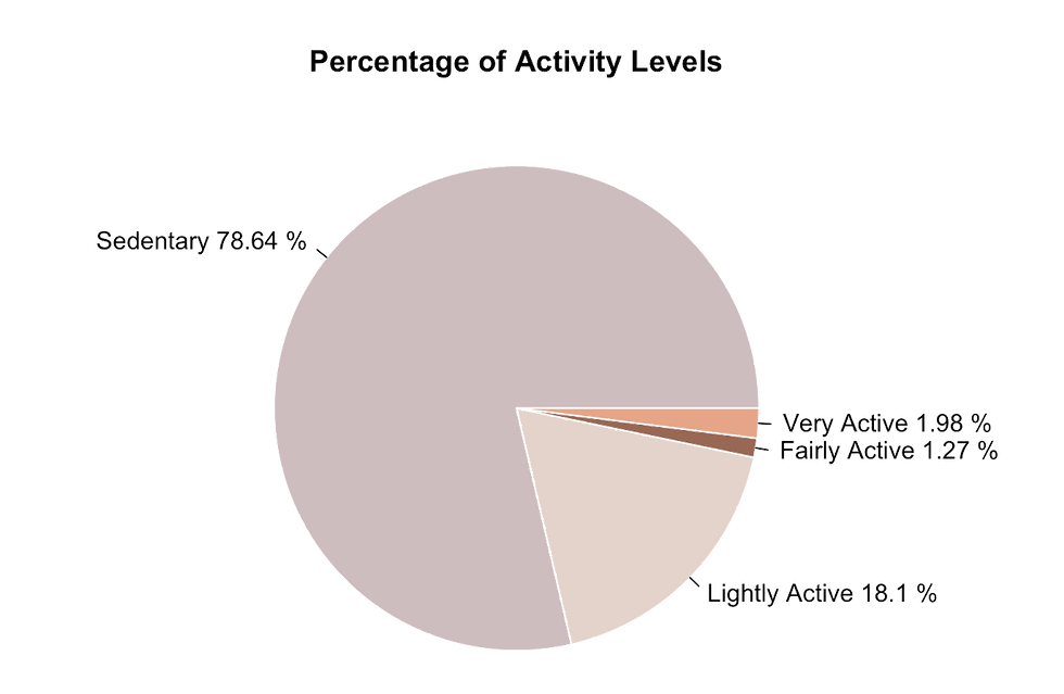
Key Findings
A significant majority, 78.64% of participants, maintained a sedentary lifestyle throughout the study period. This raises concerns, as prolonged physical inactivity often leads to various health and medical conditions, including cardiovascular disease, diabetes, and certain cancers.
Only 3.25% of participants were fairly (1.27%) and very (1.98%) physically active over the 31-day period. This low figure suggests that a minority of users utilised the Fitbit device primarily for tracking exercise, while the majority likely focused on monitoring daily habits.
It is possible that many participants are office employees or hold occupations involving predominantly sedentary activities. As per Church et al., over 80% of occupations in the US involve prolonged sitting or require light physical intensity.
Correlation between Activity Levels and Calories Burnt per Day
To explore potential correlations between activity levels and daily caloric expenditure, a visualisation will be created using ggplot2.
# Correlation between Activity Level and Calories Burnt
p1 <- ggplot(data = daily_activity_merged, aes(x = sedentary_minutes, y = calories)) + geom_point(color = "#cebdbf") + geom_smooth(method = "lm", color = "#996855", fill = "#e7a589") + xlab("Sedentary Minutes") + ylab("Calories Burnt") +
  stat_cor(method = "pearson", label.x = 500, label.y = 500) + theme_pubclean() + theme(axis.title.x = element_text(vjust = -2))
p2 <- ggplot(data = daily_activity_merged, aes(x = lightly_active_minutes, y = calories)) + geom_point(color = "#cebdbf") + geom_smooth(method = "lm", color = "#996855", fill = "#e7a589") + xlab("Lightly Active Minutes") + ylab("Calories Burnt") +
  stat_cor(method = "pearson", label.x = 200, label.y = 500) + theme_pubclean() + theme(axis.title.x = element_text(vjust = -2))
p3 <- ggplot(data = daily_activity_merged, aes(x = fairly_active_minutes, y = calories)) + geom_point(color = "#cebdbf") + geom_smooth(method = "lm", color = "#996855", fill = "#e7a589") + xlab("Fairly Active Minutes") + ylab("Calories Burnt") +
  stat_cor(method = "pearson", label.x = 50, label.y = 500) + theme_pubclean() + theme(axis.title.x = element_text(vjust = -2))
p4 <- ggplot(data = daily_activity_merged, aes(x = very_active_minutes, y = calories)) + geom_point(color = "#cebdbf") + geom_smooth(method = "lm", color = "#996855", fill = "#e7a589") + xlab("Very Active Minutes") + ylab("Calories Burnt") +
  stat_cor(method = "pearson", label.x = 60, label.y = 500) + theme_pubclean() + theme(axis.title.x = element_text(vjust = -2))

grid.arrange(p1, p2, p3, p4,
             nrow = 1,
             top = "Correlation between Activity Levels and Calories Burnt per Day"
)
Output
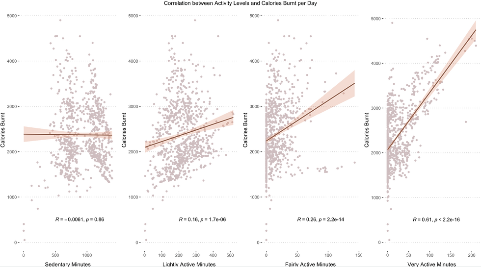
Key Findings
The less active a person is, the fewer calories they will burn.
The more active a person is, the more calories they will burn.
The correlation coefficient between Very Active Minutes and Burnt Calories is 0.61, indicating a moderate level of correlation. Additionally, with a p-value close to 0, this correlation is highly statistically significant.
Despite fairly active and very active levels representing the smallest categories, individuals in these activity levels burn more calories compared to those in sedentary and lightly active levels.
Average Hourly Physical Intensity Throughout the Day
To discern peak times of physical intensity throughout the day, a bar chart will be generated.
#Average Hourly Intensity throughout the Day
hourly_activity_merged$activity_hour_hms <- format(hourly_activity_merged$activity_hour_ymdhms, format = "%H:%M:%S")

hourly_activity_merged %>%
  group_by(activity_hour_hms) %>%
  summarise(average_hourly_intensity = mean(total_intensity)) %>%
  ggplot(aes(x = activity_hour_hms, y = average_hourly_intensity, fill = average_hourly_intensity)) +
  geom_col() +
  scale_fill_gradient(low = "#cebdbf",
                      high = "#9F7175") +
  labs(x = "Time of Day", y ="Average Intensity", title ="Average Hourly Intensity throughout the Day")+
  guides(fill = guide_legend(title="Average Hourly Intensity")) +
  theme_pubclean() +
  theme(plot.title = element_text(hjust = 0.5, vjust = 0.8, size = 16)) +
  theme(axis.text.x = element_text(angle = 90))
Output
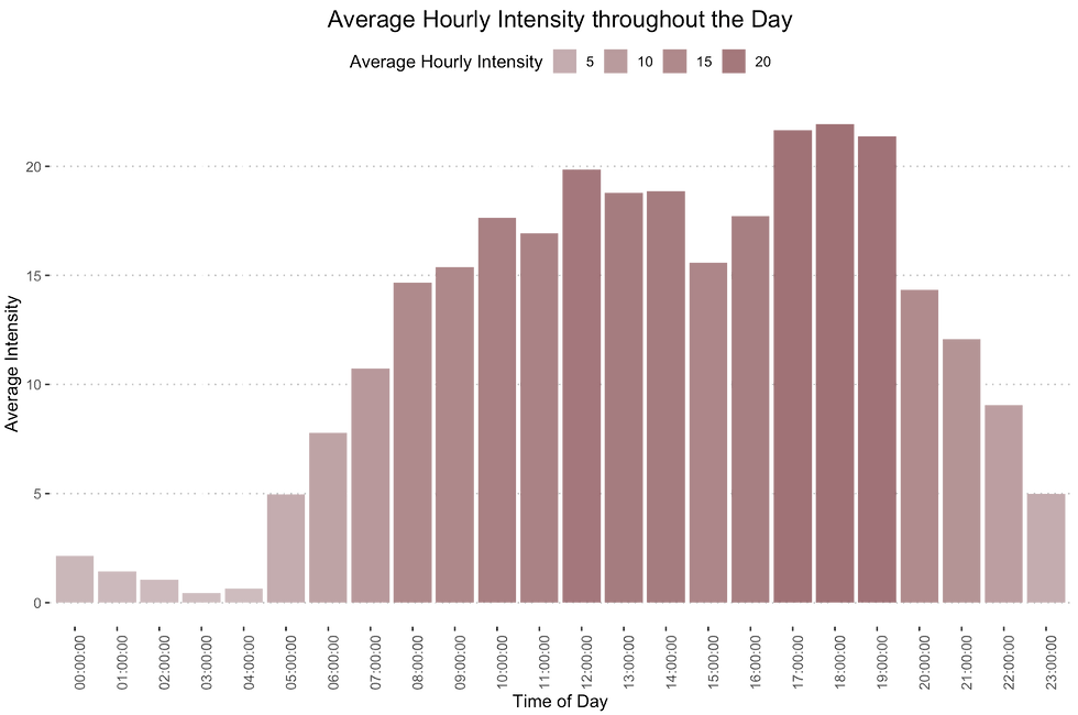
Key Findings
The lowest physical intensities occur from 23:00 to 5:00, corresponding to typical sleeping hour.
Peak intensity is observed from 17:00 to 19:00, coinciding with the time when people usually return home from work.
Another peak in intensity is observed from 12:00 to 14:00, indicative of lunch breaks.
Average Physical Intensity Throughout the Week
To determine the most active day of the week, a weekly bar chart was generated.
#Average Intensity Throughout the Week
hourly_activity_merged$weekday <- factor(hourly_activity_merged$weekday, levels=c("Monday", "Tuesday", "Wednesday", "Thursday", "Friday", "Saturday", "Sunday"))

hourly_activity_merged %>%
  group_by(weekday) %>%
  summarise(average_intensity = mean(total_intensity)) %>%
  ggplot(aes(x = weekday, y = average_intensity, fill = average_intensity)) +
  geom_col() +
  scale_fill_gradient(low = "#cebdbf",
                      high = "#9F7175") +
  labs(x = "Day of Week", y ="Average Intensity", title ="Average Intensity throughout the Week")+
  guides(fill = guide_legend(title="Average Intensity")) +
  theme_pubclean() +
  theme(plot.title = element_text(hjust = 0.5, vjust = 0.8, size = 16)) +
  theme(axis.text.x = element_text(angle = 90))
Output
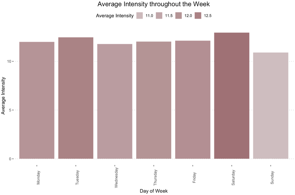
Key Findings
Saturday emerges as the most active day, likely due to more free time.
An unexpected peak in activity is observed on Tuesday, while intensity levels on other weekdays reamin relatively consistent.
Sunday shows the lowest activity levels, possibly due to individuals taking rest before the start of the workweek.
Average Hourly Physical Intensity throughout the Week
Below, the average hourly intensity for each day of the week is presented, offering further insights into intensity levels over the week.
# Average Hourly Intensity throughout the Week
hourly_activity_merged %>%
  group_by(weekday, activity_hour_hms) %>%
  summarise(average_hourly_intensity = mean(total_intensity)) %>%
  ggplot(aes(x = activity_hour_hms, y = weekday, fill = average_hourly_intensity)) +
  theme(axis.text.x = element_text(angle=90)) +
  scale_fill_continuous(low="white", high = "#9F7175") +
  geom_tile(colour = "white", lwd= .5, linetype = 1) +
  coord_fixed() +
  labs(x = "Time of Day", y ="Weekday", title ="Average Hourly Intensity throughout the Week", fill = "Average Hourly Intensity") +
  theme(plot.title = element_text(hjust = 0.5, vjust = 0.8, size = 16), panel.background = element_blank())
Output
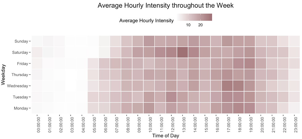
Key Findings
Consistent with earlier observations, intensity peaks from 17:00 to 19:00, post-work hours.
The midday peak from 12:00 to 14:00 on weekdays (Monday - Friday) is less pronounced than the previous graph had shown. The peak during that period actually comes from high activity and intensity levels on Saturday when people have more time to workout or do other activities that require higher intensities.
Users go to bed and wake up later during weekends.
4.2.2 Device Usage Levels
Daily usage of the device will be examined to understand how users use the device and how often they use it.
Daily Device Usage Percentage
To determine device usage frequency, participants will be categorized based on the number of days they used the device. The resulting percentages will be visualised using a pie chart.
activity_usage <- daily_activity_merged %>%
  group_by(id) %>%
  summarize(days_used = sum(n())) %>%
  mutate(daily_usage_level = case_when(
    days_used >= 1 & days_used <= 10 ~ 'Low Usage',
    days_used > 10 & days_used <= 20 ~ 'Moderate Usage',
    days_used > 20 ~ 'High Usage'
  )) %>%
  drop_na() %>%
  group_by(daily_usage_level) %>%
  summarize(users_total = n())

head(activity_usage)
Output
# A tibble: 3 × 2
  daily_usage_level    users_total
  <chr>                <int>
1 High Usage              24
2 Low Usage                1
3 Moderate Usage           8
# Daily Device Usage Percentage
slices_v2 <- c(1, 8, 24)
labels_v2 <- c("Low Usage", "Moderate Usage", "High Usage")
pct <- slices_v2/sum(slices_v2)*100
pct <- round(pct, 2)
labels_v2 <- paste(labels_v2, pct)
labels_v2 <- paste(labels_v2, "%", sep = "")
colours <- c("#996855", "#e7a589", "#cebdbf")
pie(slices_v2, labels = labels_v2,
main="Daily Usage Levels",
col = colours,
border = "white",
cex = 0.7)
legend('topright', c("Low Usage: 1 - 10 days","Moderate Usage: 11 - 20 days","High Usage: 21 - 31 days"), cex = 0.7, fill = colours)Output
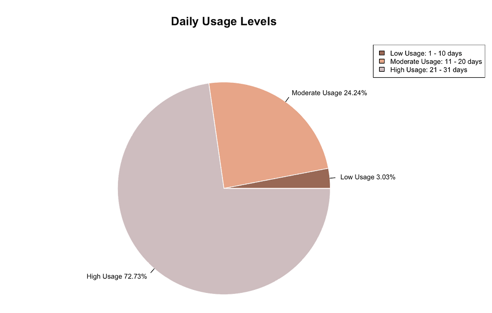
Key Findings
The majority of participants (72.73%) used their device very frequently (21 - 31 days).
24.24% of participants used the device frequently (11 -20 days).
Only 3.03% of participants had low device usage (1 - 20 days).
Device Worn in a Day Percentage
The pie chart below illustrates the percentage with which the device was worn all day.
daily_activity_merged$device_worn <- daily_activity_merged$sedentary_minutes + daily_activity_merged$fairly_active_minutes + daily_activity_merged$lightly_active_minutes + daily_activity_merged$very_active_minutes
daily_activity_merged$device_worn <- daily_activity_merged$device_worn/60
daily_activity_merged$device_worn_24 <- daily_activity_merged$device_worn == 24
device_worn <- count(daily_activity_merged, device_worn_24) %>%
  drop_na()

glimpse(device_worn)
Output
Rows: 2
Columns: 2
$ device_worn_24 <lgl> FALSE, TRUE
$ n              <int> 458, 378
slices_v3 <- c(378, 458)
labels_v3 <- c("Worn all day", "Not worn all day")
pct_v1 <- slices_v3/sum(slices_v3)*100
pct_v1 <- round(pct_v1, 2)
labels_v3 <- paste(labels_v3, pct_v1)
labels_v3 <- paste(labels_v3, "%", sep = "")
colours <- c("#996855", "#cebdbf")
pie(slices_v3, labels = labels_v3,
main="Percentage of the Device Being Worn the Whole Day", col = colours, border = "white")Output
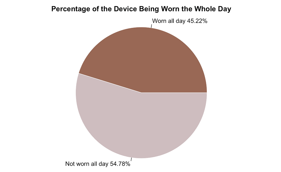
Key Findings
54.78% of participants did not wear the device for the entire day.
The Number of Hours the Device was Worn Throughout the Week
Given that over 50% of participants did not wear the device for the entire 24 hours per day, it is pertinent to examine the number of hours the device was worn per day.
# How Many Hours was the Device Worn per Day
device_worn_24_7 <- daily_activity_merged[c("id", "weekday", "device_worn", "activity_date_ymd")]
device_worn_24_7$weekday <- factor(device_worn_24_7$weekday, levels = c("Monday", "Tuesday", "Wednesday", "Thursday", "Friday", "Saturday", "Sunday"))

device_worn_24_7 %>%
  drop_na() %>%
  ggplot(aes(y = device_worn, x = weekday, group = 1)) +
  geom_point(color = "#cebdbf", size = 1) +
  geom_smooth(method = "loess", span = 0.2, color = "#996855", fill = "#e7a589") +
  coord_cartesian(ylim = c(0, 24)) +
  ggtitle("The Number of Hours the Device was Worn throughout the Week")+
  ylab("The Number of Hours Worn within a Day") +
  xlab("Day of Week") +
  theme_pubclean() +
  theme(axis.text.x = element_text(angle = 90), plot.title = element_text(hjust = 0.5))
Output
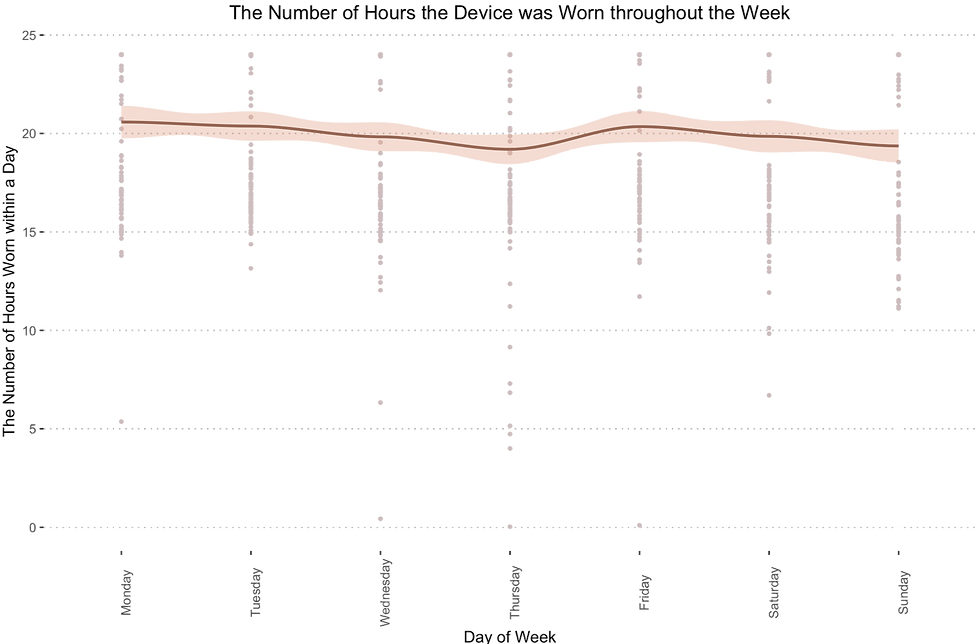
It appears that many participants wore the tracker for less than 20 hours per day. To determine the exact percentage of how many times the device was worn for less than 20 hours per day, the count() function will be used and a pie chart will be created.
# Count of the device being worn < 20 hours
worn_less_20 <- daily_activity_merged %>%
  count(device_worn < 20) %>%
  drop_na()

head(worn_less_20)
Output
  device_worn < 20   n
1            FALSE 433
2             TRUE 403
# Percentage of the device being worn < 20 hours
slices_v3 <- c(403, 433)
labels_v3 <- c("Device worn < 20 hours", "Device worn > 20 hours")
pct_v1 <- slices_v3/sum(slices_v3)*100
pct_v1 <- round(pct_v1, 2)
labels_v3 <- paste(labels_v3, pct_v1)
labels_v3 <- paste(labels_v3, "%", sep = "")
colours <- c("#996855", "#cebdbf")
pie(slices_v3, labels = labels_v3,
main="Percentage of the Device Being Worn Less than 20 Hours per Day", col = colours, border = "white")Output
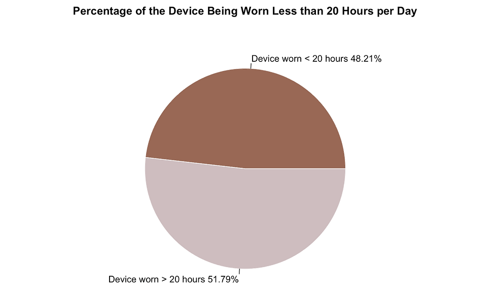
Key Findings
A significant portion of participants did not wear the device for the entire day during the study.
48.21% of participants wore the device for less than 20 hours per day.
Activity Device Usage vs Sleep Device Usage
Given that almost half of the participants wore the device for less than 20 hours per day, it is plausible that these unaccounted hours correspond to sleep periods when users may remove the device for comfort. To investigate this hypothesis, two bar graphs will be plotted comparing activity usage levels (users tracking their daily activity) and sleep usage levels (users tracking their sleep).
# Activity usage per participant
activity_usage_v2 <- clean_daily_calories %>%
  group_by(id) %>%
  count() %>%
  arrange(n) %>%
  mutate(activity_percentage = (n/31)*100)
head(activity_usage_v2)

p5 <- ggplot(activity_usage_v2, aes(x = reorder(id, n), y = activity_percentage)) +
  geom_col(fill = "#cebdbf")  +
  labs(title="Activity Device Usage", x = "Particpant #", y = "Percentage of Logged Activity", caption = "33 participants") +
  theme_pubclean() +
  theme(plot.title = element_text(hjust = 0.5, vjust = 0.8, size = 12)) +
  theme(axis.text.x = element_text(angle = 90, size = 7)) +
  theme(axis.title.x = element_text(size = 10)) +
  theme(axis.title.y = element_text(size = 10)) +
  theme(plot.caption = element_text(size = 7))

# Sleep usage per participant
sleep_usage <- clean_daily_sleep %>%
  group_by(id) %>%
  count() %>%
  arrange(n) %>%
  mutate(sleep_percentage = (n/31)*100) #% of nights users monitored sleep
head(sleep_usage)

p6 <- ggplot(sleep_usage, aes(x= reorder(id, n), y = sleep_percentage)) +
  geom_col(fill = "#cebdbf") +
  labs(title="Sleep Device Usage", x= "Particpant #", y="Percentage of Logged Sleep", caption = "24 participants") +
  theme_pubclean() +
  theme(plot.title = element_text(hjust = 0.5, vjust = 0.8, size = 12)) +
  theme(axis.text.x = element_text(angle = 90, size = 7)) +
  theme(axis.title.x = element_text(size = 10)) +
  theme(axis.title.y = element_text(size = 10)) +
  theme(plot.caption = element_text(size = 7))

grid.arrange(p5, p6,
             ncol = 1,
             top = "Activity Device Usage vs Sleep Device Usage"
)
Output
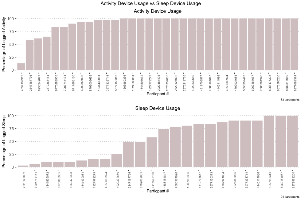
Key Findings
33 participants tracked their daily activity, whereas 24 participants tracked their sleep. This indicates that all participants tracked their daily activity, but 9 of them did not track their sleep.
Over 21 participants wore the device throughout the whole day to track their daily activity, but only 3 wore it to bed consistently during the study. This suggests that many users remove their Fitbit tracker before sleeping.
Section 5: Act
In this section, recommendations will be provided based on the findings. It will be divided into sub-sections following the guiding questions that were provided at the beginning of this project:
What are the current trends in smart device usage?
How do these trends relate to Bellabeat's target customers?
How can these trends influence Bellabeat's marketing strategy?
5.1 Smart Device Usage Trends
Activity and Intensity Levels
The average total steps per day (8,518), fall below the recommended 10,000 steps per day.
Very high sedentary time (nearly 16 hours) can lead to multiple health issues. It was suggested that many users of the Fitbit device are professionals who do jobs which mostly involve sedentary behaviour.
The more active a person is, the more calories they burn. The less active a person is and the longer they stay in a sedentary position, the fewer calories they burn.
Only 3.25% of participants were fairly and very physically active with an average of 19.47 minutes per day. This low figure suggests that not many users might be using the Fitbit device to track exercise; rather, they might be tracking daily habits.
During the weekday, the highest intensity is predominately from 17:00 to 19:00 when people usually go home from work.
During the weekend, the peak in intensity and high activity is on Saturday afternoon when people have more time to work out or do other activities that require higher intensities. However, on Sunday, users are less active as they tend to treat Sunday as a rest day.
Device Usage Levels
Most participants (72.73%) used the device very frequently for 21 - 31 days.
However, 54.78% of the participants did not wear the device for the entire day.
48.21% of the participants wore the device less than 20 hours per day.
The majority tracked their daily activity but did not monitor their sleep.
5.2 Applying the Trends to Bellabeat Customers
Activity and Intensity Levels
Working professionals: Results suggest that Fitbit users are mostly working professionals as the highest intensity during the weekday is around 18:00, correlating to the time when people usually finish their work and go home. → Many Bellabeat customers are also working professionals.
Mental health problems and eating disorders: There is a very high sedentary time, and the average number of total steps is less than the amount recommended by health experts. This corresponds to the information above suggesting that most users were office workers or working professionals who simply did not find much time to workout due to their busy schedule. It has been proposed that excessive sedentary time is associated with mental health issues including depression, anxiety, and self-esteem. → Since the target market is female working professionals, this information is especially important as women are three times more likely than men to experience common mental health problems and eating disorders.
Device Usage Levels
Quality of Sleep: Many Fitbit users voiced out that it is uncomfortable to wear the tracker to bed and that they would rather save some battery or recharge the device during the bedtime. Some Fitbit users also mentioned that they do not find the sleep data useful. These might be some of the reasons why not all users wore the tracker to bed and monitor their sleep. However, as per Eatough: "The amount and quality of sleep ... have a lasting impact on you when you’re awake. It affects your mental fitness, physical well-being, and even your risk of developing lifestyle diseases." → This is essential for the Bellabeat customers who might not be getting enough sleep which can not only impact their job performance but their wellness overall.
5.3 Bellabeat Marketing Strategy Recommendations
Recommendations were made based on the data analysis results that would benefit and target the female professionals. The recommendations are aimed to improve Bellabeat's Ivy health tracker.
5.3.1 Target Market
The target market for this marketing strategy is female working professionals who aim to support their mental health while staying fit. Their focus is not necessarily to optimise their fitness and workout performance, rather to prioritise their mental and reproductive health by staying physically active and healthy amid their busy schedule.
5.3.2 Recommendations for Product Improvement
Personalised Workout Schedule for Female Working Professionals
Many Bellabeat customers are working professionals who might often be too busy to engage in regular exercise. Studies propose that people with fewer opportunities for daily workouts during their work week can either workout for longer periods during the weekends and/or work for shorter periods during the week to maintain the recommended 75 - 150 minutes of moderate to vigorous activity a week. Bellabeat can provide personalised workout schedules that would not only reach the recommended amount of activity but also accommodate the user's busy schedule.
Gentle Reminders and Inactivity Alerts
To reduce the amount of sedentary time, Bellabeat added the inactivity alert feature which sends out alerts to the users when they have been inactive for too long, to remind them to get up and move around. This feature, however, is only available to Leaf and Time but not the Ivy tracker. Since Ivy focuses on wellness, vibrations and reminders might be too distracting which can induce anxiety. Instead, Ivy allows users to set their own daily goals for steps and activity to motivate them to make better choices for their health. However, knowing that the target market are female professionals who might be involved in daily prolonged sitting, gentle inactivity alerts should still be an option as high sedentary behaviour has negative health effects.
5.3.3 Recommendations for Marketing Strategies
Bellabeat offers a personalised holistic wellness approach to health compared to companies such as Fitbit that are more fitness and performance-oriented. This gives Bellabeat a competitive edge as this holistic approach might be valued by female professionals who, according to Priory (2023), are more likely to experience work-related stress.
Based on the analysis of this project, Bellabeat's marketing strategy should focus on the following aspects of the Ivy wellness tracking device:
Detailed Sleep Analysis
Bellabeat Ivy provides a detailed sleep analysis with a score that is going to help guide users to make smarter, healthier decisions that would work with their body and mind. The marketing team should stress the importance of sleep as it is vital to our health and getting enough sleep keeps the body and mind in optimal condition and ready for the day. Since the working environment can be sometimes stressful and challenging, having a regular sleep routine and good night sleep is very important as it "restores the body, improves concentration, regulates mood, and sharpens judgement and decision-making." Having adequate sleep was proven to drastically reduce feelings of anxiety and improve the ability to process stress. Tracking sleep can help with maintaining a regular sleep schedule or diagnose and rectify sleep issues.
Comfortable and Lightweight
Despite the importance of sleep tracking, some Fitbit users took off their tracking device during the night as they found it uncomfortable to sleep with. The marketing team should emphasise that Bellabeat Ivy is incredibly lightweight making it very comfortable to wear anywhere and anytime including to bed.
Strong Battery Life
Bellabeat Ivy also boasts a long battery life that can last up to 8 days. Therefore, users would have to worry less about recharging the device overnight.
Conclusion
The purpose of this case study was to identify potential growth opportunities for Bellabeat, a wellness company, and improve their marketing strategy by analysing smart device usage among Fitbit consumers. Based on the analysis conducted, it can be concluded that the majority of fitness smart device users are working professionals who lack the recommended active minutes as they are often too busy to engage in regular exercise. Therefore, it is recommended to tailor Bellabeat's marketing strategies and products to working professionals by providing personalised workout schedules as well as implementing gentle inactivity alerts. Moreover, it was suggested to emphasise the importance of sleep because of its numerous benefits. These are the recommendations and conclusions drawn from the analysis of the Fitbit data. However, further analysis into other smart device companies such as the Apple Watch or Garmin is advised to support these results and provide additional insight into Bellabeat's strategies.
Comments